20. Pretraining

Authors:

Heta Gandhi & Sam Cox

Up until this point, we have been building deep learning models from scratch and mostly training on labelled data to complete a task. A lot of times, especially in chemistry, labelled data is not readily accessible or abundant. In this scenerio, it is helpful to use a pretrained model and leverage the pretrained weights and architecture to learn a new task. In this chapter, we will look into pretraining, how it works, and some applications.

Audience & Objectives

This chapter builds on Standard Layers and Graph Neural Networks. After completing this chapter, you should be able to

• Understand why pretraining is useful, and in which situations it is appropriate

• Understand transfer learning and fine-tuning

• Be able to use a pretrained model for a simple downstream task

20.1. How does pretraining work?

Pretraining is a training process in which the weights of a model can be trained on a large dataset, for use as a starting place for training on smaller, similar datasets.

Supervised deep learning models are generally trained on labeled data to achieve a single task. However, for most practical problems, especially in chemistry, labeled examples are limited, imbalanced, or expensive to obtain, whereas unlabeled data is abundant. When labeled data is scarce, supervised learning techniques lead to poor generalization [Mao20]. Instead, in low data regimes, self-supervised learning (SSL) methods (an unsupervised learning approach) are often employed. In SSL, the model is trained on labels that are automatically generated from the data itself. SSL has been largely successful in large language models and computer vision, as well as in chemistry. SSL is the approach used to pre-train models, which can be fine-tuned for downstream tasks, or can be used for transfer learning. The figure below from [ECBV10] shows how pretraining can affect test error.

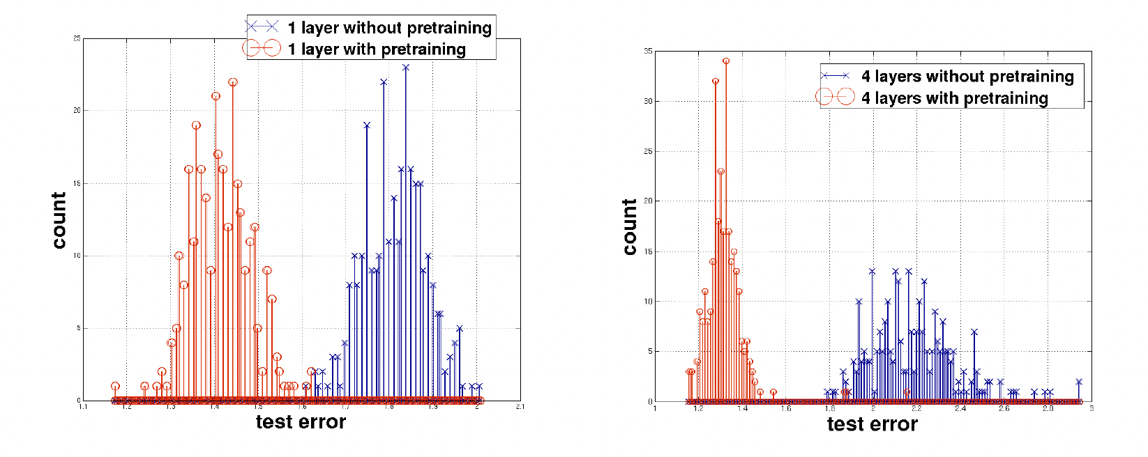
Fig. 20.1 Test error comparison. Comparing test loss error on MNIST data, with 400 different iterations each. On the left, red and blue correspond to test error for one layer with and without pretraining, respectively. The right image has four layers instead of one.

20.2. Why does pretraining a model work?

There are many theoretical reasons for why pretraining works. Pretraining can be seen as a sort of regularization technique, because it initializes parameters and restricts learning to a subset of the parameter space [Mao20, ECBV10]. More specifically, the parameters are initialized so that they are restricted to a better local basin of attraction…a region that captures the structure of the input distribution [YCS+20]. Practically, the parameter space is more constrained as the magnitude of the weights increase during training because the function becomes more nonlinear, and the loss function becomes more topologically complex [YCS+20].

In plainer words, the model collects information about which aspects of the inputs are important, setting the weights accordingly. Then, the model can perform implicit metalearning (helping with hyperparameter choice), and it has been shown that the fine-tuned models’ weights are often not far from the pretrained values [Mao20]. Thus, pretraining can help your model drive the parameters toward the values you actually want for your downstream task.

20.3. Transfer learning vs fine-tuning

20.3.1. Transfer Learning

Transfer learning works by taking a pretrained model and freezing the layers and parameters that were already trained. Then you can either add layer(s) on top, or you can modify only the last layer and train it to your new task. In transfer learning, the feature extraction layers from the pretraining process are kept frozen. It is necessary that your data has some connection with the original data.

There are largely two types of transfer learning, and you can find a more formal definition in [Mao20]. The first is transductive transfer learning, where you have the same tasks, but only have labels in the source (pretraining) dataset. For example, imagine training a model to predict the space group of theoretical inorganic crystal structures. Transductive transfer learning could be using this model to predict the space group of self-assembled biochemical structures. You’re using a different dataset, where the only labels are in the inorganic crystal data.

The second type of transfer learning is called inductive transfer learning, where you want to learn a new task, and you have labels for both your source and your target dataset. For example, imagine you train a model to predict solubility of small organic molecules. You could use inductive transfer learning and use this model to predict the pKa of another organic molecule (labeled) dataset. Notice that in both cases, the input type is the same for the source and the target problem. Also, this shouldn’t be too difficult for the model, since you would imagine there would be some relationship between the solubility and the pKa of organic molecules.

20.3.2. Fine-Tuning

Fine-tuning is a bit different in that instead of freezing the layers and parameters, you retrain either the entire model or parts of the model. So instead of freezing the pre-trained parameters, you use them as a starting point. This can be especially helpful for low-data regimes. However, it is easy to quickly overfit when fine-tuning a pretrained model, especially on a relatively small dataset, so it is important to tune your hyperparameters, such as the learning rate.

For example, SMILES-BERT [WGW+19] is a model pre-trained on SMILES strings via a recovery task. The unlabeled data is SMILES strings, with randomly masked or corrupted tokens. The model is trained to correctly recover the original SMILES string. By learning this task, the model learns to identify important components of the input, which can be applied via fine-tuning to a molecular property prediction downstream task. In this case, the original dataset is unlabeled, and the labels are generated automatically from the data, which is SMILES strings. Then, the target task dataset is SMILES strings with a molecular property label.

For more information on the comparison between transfer learning and fine-tuning, you can check out this youtube video. Also, the figure below gives a layout of fine-tuning and transfer learning. What is important to note is that in transfer learning, we retrain the last layer or add layers on the end, whereas in fine-tuning we can retrain the feature extraction layers also.

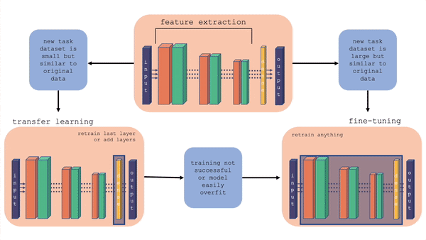
Fig. 20.2 Comparison of fine-tuning and transfer learning with a general model architecture. Starting with the top middle block (original model), follow the flow chart for different situations.

20.4. Pretraining for graph models

GNNs typically require a large amount of labeled data and are not typically generalizable. Particularly in chemistry, there is a significant amount of unlabeled graph data available. Because of this, SSL has become very popular in GNNs, and it can be broadly split into two categories based on the method: contrastive learning and predictive learning. Predictive models are trained to generate labels based on the input, whereas contrastive models learn to generate diverse and informative information about the input and perform contrastive learning (compare representations) [ZLW+21]. You can see a comparison of the two methods and example architectures in the figure below [XXZ+22].

Contrastive learning is focused on learning to maximize the agreement of features among differently augmented views of the data [YCS+20]. The goal of a contrastive learning approach is for the model to learn representations invariant to the perturbations or augmentations by maximizing the agreement between the base graph and its augmented versions. In other words, if two graphs are similar, the representation should be similar. Likewise, if two graphs are dissimilar, the model learns that the representations should be dissimilar. There have been many approaches to this, including subgraph or motif-based learning, where the model learns to break apart frequent subgraph patterns, such as functional groups [ZLW+21]. Another approach by [YCS+20] combined 4 different data augmentation techniques, similar to how masking is done for large language models, though [SXW+21] found that those random augmentations often changed the global properties of the molecular graph, proposing instead to augment by replacing substructures with bioisosteres.

Another way to think about contrastive learning is that the model looks at one or more encoders and learns that similar graphs should output similar representations, while less similar graphs should have less agreeable representations. Contrastive learning frameworks construct multiple views of each input graph, then an encoder outputs a representation for each view [XXZ+22]. During training, the encoder is trained so that the agreement between representations of the same graph is maximized. In this case, representations from the same instance (same graph) should agree, while representations from separate instances should disagree. The agreement is often measured with Mutual Information, which is a measure of shared information across representations. A thorough discussion of agreement metrics is given in [XXZ+22].

Predictive models, in contrast, train with self-generated labels. This category of model is sometimes called generative models, as graph reconstruction is a popular approach. In graph reconstruction, the graph is distorted in some way (node removed, edge removed, node replaced with another type, etc.), and the model learns to reconstruct the original graph as its output. However, it is not correct to think of predictive models as simply generative models, because graph reconstruction, with an encoder and decoder, is not the only type of predictive model for graphs. Another popular example is property prediction. In property prediction examples, remember that we are still training on unlabeled data, so the property needs to be something implicit in the data, such as the connectivity of two nodes {cite} xie2022self. There won’t be a decoder in this case, because we don’t want a graph as the output.

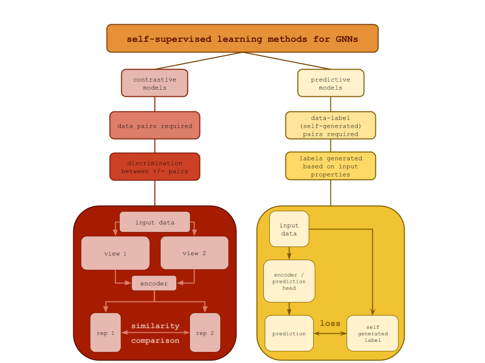
Fig. 20.3 Comparison of contrastive and predictive models in the context of self-supervised learning for GNNs. On the left, contrastive models require data pairs and discriminate between positive and negative examples, and an example architecture is provided. On the right, predictive models have data(self)-generated labels and predict outputs based on input properties. An example architecture is provided.

20.5. Running This Notebook

Click the    above to launch this page as an interactive Google Colab. See details below on installing packages.

Tip

To install packages, execute this code in a new cell.

!pip install dmol-book

If you find install problems, you can get the latest working versions of packages used in this book here

Let’s look at a simple example of using a pre-trained model to do transfer learning. We will load a pre-trained model from the huggingface library and use it to predict aqueous solubility of molecules. HuggingFace is an open source platform that enables users to build, train and deploy their deep learning models. We load the ChemBERTa model which was originally trained on SMILES strings from the ZINC-250k dataset. Using the learned representations from ChemBERTa, we can predict aqueous solubility on a smaller dataset.[SKE19]

from simpletransformers.classification import ClassificationModel
import pandas as pd, sklearn, matplotlib.pyplot as plt, numpy as np

We begin by creating our train and test datasets. The BBB dataset that we use is slightly imbalanced, so we use stratification to make sure both classes are present in train and test sets.

soldata = pd.read_csv(
    "https://github.com/whitead/dmol-book/raw/main/data/curated-solubility-dataset.csv"
)

N = int(len(soldata) * 0.1)
sample = soldata.sample(N, replace=False)
train = sample[: int(0.8 * N)]
test = sample[int(0.8 * N) :]

train_dataset = train[["SMILES", "Solubility"]]
train_dataset = train_dataset.rename(columns={"Solubility": "labels", "SMILES": "text"})
test_dataset = test[["SMILES", "Solubility"]]
test_dataset = test_dataset.rename(columns={"Solubility": "labels", "SMILES": "text"})

Next, we initialize a classification model for ChemBERTa_zinc250k_v2_40k pre-trained model. ClassificationModel is a binary classification model by default, so we specify that we want to do regression. This will basically change the layer layer of the original model to output regressed values rather than classification probabilities. Then we train the model using the solubility dataset.

model = ClassificationModel(
    "roberta",
    "seyonec/ChemBERTa_zinc250k_v2_40k",
    num_labels=1,
    args={
        "num_train_epochs": 5,
        "regression": True,
        "use_multiprocessing": False,
        "use_multiprocessing_for_evaluation": False,
    },
    use_cuda=False,
)

Some weights of the model checkpoint at seyonec/ChemBERTa_zinc250k_v2_40k were not used when initializing RobertaForSequenceClassification: ['lm_head.bias', 'lm_head.dense.weight', 'roberta.pooler.dense.bias', 'lm_head.dense.bias', 'lm_head.decoder.bias', 'roberta.pooler.dense.weight', 'lm_head.decoder.weight', 'lm_head.layer_norm.bias', 'lm_head.layer_norm.weight']
- This IS expected if you are initializing RobertaForSequenceClassification from the checkpoint of a model trained on another task or with another architecture (e.g. initializing a BertForSequenceClassification model from a BertForPreTraining model).
- This IS NOT expected if you are initializing RobertaForSequenceClassification from the checkpoint of a model that you expect to be exactly identical (initializing a BertForSequenceClassification model from a BertForSequenceClassification model).

Some weights of RobertaForSequenceClassification were not initialized from the model checkpoint at seyonec/ChemBERTa_zinc250k_v2_40k and are newly initialized: ['classifier.out_proj.bias', 'classifier.dense.weight', 'classifier.dense.bias', 'classifier.out_proj.weight']
You should probably TRAIN this model on a down-stream task to be able to use it for predictions and inference.

model.train_model(
    train_df=train_dataset,
    args={"num_train_epochs": 5},
)

(500, 1.9525295648798346)

Now we evaluate the trained model on our test set.

result, model_outputs, wrong_predictions = model.eval_model(
    test_dataset, acc=sklearn.metrics.mean_squared_error
)
print(result)

{'acc': 1.6435277972218296, 'eval_loss': 1.6435277891159057}

# make predictions and see how we do
predictions = model.predict(test_dataset["text"].tolist())[0]

# plot the predictions
plt.scatter(test_dataset["labels"].tolist(), predictions, color="C0")
plt.plot(test_dataset["labels"], test_dataset["labels"], color="C1")
plt.text(
    -10,
    0.0,
    f"Correlation coefficient: {np.corrcoef(test_dataset['labels'], predictions)[0,1]:.3f}",
)
plt.xlabel("Actual Solubility")
plt.ylabel("Predicted Solubility")
plt.show()

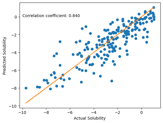
The model performs quite well on our test set. We have fine-tuned the pretrained model for a task that it was not trained for. This shows that even though the original model was trained on the ZINC dataset, the input representations can be used to make predictions on another dataset, with a different task. Using pre-trained models saves time and effort spent in training the model. To further improve performance on this silubility prediction task, you can change some other parameters like the learning rate or add additional layers before the output layer.

20.6. Cited References

SKE19

Murat Cihan Sorkun, Abhishek Khetan, and Süleyman Er. AqSolDB, a curated reference set of aqueous solubility and 2D descriptors for a diverse set of compounds. Sci. Data, 6(1):143, 2019. doi:10.1038/s41597-019-0151-1.

Mao20(1,2,3,4)

Huanru Henry Mao. A survey on self-supervised pre-training for sequential transfer learning in neural networks. arXiv preprint arXiv:2007.00800, 2020.

ECBV10(1,2)

Dumitru Erhan, Aaron Courville, Yoshua Bengio, and Pascal Vincent. Why does unsupervised pre-training help deep learning? In Proceedings of the thirteenth international conference on artificial intelligence and statistics, 201–208. JMLR Workshop and Conference Proceedings, 2010.

YCS+20(1,2,3,4)

Yuning You, Tianlong Chen, Yongduo Sui, Ting Chen, Zhangyang Wang, and Yang Shen. Graph contrastive learning with augmentations. Advances in Neural Information Processing Systems, 33:5812–5823, 2020.

WGW+19

Sheng Wang, Yuzhi Guo, Yuhong Wang, Hongmao Sun, and Junzhou Huang. Smiles-bert: large scale unsupervised pre-training for molecular property prediction. In Proceedings of the 10th ACM international conference on bioinformatics, computational biology and health informatics, 429–436. 2019.

ZLW+21(1,2)

Zaixi Zhang, Qi Liu, Hao Wang, Chengqiang Lu, and Chee-Kong Lee. Motif-based graph self-supervised learning for molecular property prediction. Advances in Neural Information Processing Systems, 34:15870–15882, 2021.

XXZ+22(1,2,3)

Yaochen Xie, Zhao Xu, Jingtun Zhang, Zhengyang Wang, and Shuiwang Ji. Self-supervised learning of graph neural networks: a unified review. IEEE Transactions on Pattern Analysis and Machine Intelligence, 2022.

SXW+21

Mengying Sun, Jing Xing, Huijun Wang, Bin Chen, and Jiayu Zhou. Mocl: data-driven molecular fingerprint via knowledge-aware contrastive learning from molecular graph. In Proceedings of the 27th ACM SIGKDD Conference on Knowledge Discovery & Data Mining, 3585–3594. 2021.