7. Standard Layers#
We will now see an overview of the enormous diversity in deep learning layers. This survey is necessarily limited to standard layers and we begin without considering the key layers that enable deep learning of molecules and materials. Almost all the layers listed below came out of a model for a specific task and were not thought-up independently. That means that some of the layers are suited to specific tasks and often the nomenclature around that layer is targeted towards a specific kinds of data.
Audience & Objectives
This chapter builds on the overview from Deep Learning Overview and Regression & Model Assessment. After completing this chapter, you should be able to:
Construct a neural network with various layers
Understand how layers change shapes
Recognize hyperparameters in a neural network
Split data into train, test, and validation
Regularize to prevent overfitting
The most common type is image data and we first begin with an overview of how image features are represented. Generally, an image is a rank 3 tensor with shape \((H, W, C)\) where \(H\) is the height of the image, \(W\) is the width, and \(C\) is the number of channels (typically 3 – red, green, blue). Since all training is in batches, the input features shape will be \((B, H, W, C)\). Often layers will discuss input as having a batch axis, some number of shape axes, and then finally a channel axis. The layers will then operate on perhaps only the channels or only the shape dimensions. The layers are all quite flexible, so this is not a limitation in practice, but it’s important to know when reading about layer types. Often the documentation or literature will mention batch number or channels and this is typically the first and last axes of a tensor, respectively.
Note
Everything and nothing is batched in deep learning. Practically, data is always batched. Even if your data is not batched, the first axis input to a neural network is of unspecified dimension and called the batch axis. Many frameworks make this implicit, meaning if you say the output from one layer is shape \((4,5)\), it will be \((B, 4, 5)\) when you actually inspect data. Or, for example in JAX, you can write your code without batching and make it batched through a function transform. So, all data is batched but often the math, frameworks, and documentation make it seem as if there is no batch axis.

Fig. 7.1 A typical neural network architecture is composed of multiple layers. This network is used to classify images.#
An example of what a neural network looks like is shown in Fig. 7.1. In this case, its input is a 128x128 images with 3 channels (red, green, blue) and it outputs is a vector of probabilities of length 128 that indicate the class of the images. In other words, it takes in an image and gives it a probability of 128 possible labels like “cat” or “vase” or “crane”. The words annotating the figure indicate the different layer types we’ll learn about below.
7.1. Hyperparameters#
We saw from the Full connected (FC)/Dense layer that we have to choose if we use bias, choose the activation function, and choose the output shape. As we learn about more complex layers, there will be more choices. These choices begin to accumulate and in a neural network you may have billions of possible combinations of them. These choices about shape, activation, initialization, and other layer arguments are called hyperparameters. They are parameters in the sense that they can be tuned, but they are not trained on our data. So we call them hyperparameters to distinguish them from the “regular” parameters like value of weights and biases in the layers. The name is inherited from Bayesian statistics.
Choosing these hyperparameters is difficult and we typically rely on the body of existing literature to understand ranges of reasonable parameters. In deep learning, we usually are in a regime of hyperparameters which yield many trainable parameters (deep networks) and thus our models can represent any function. Our models are expressive. However, optimizing hyperparameters makes training faster and/or require less data. For example, papers have shown that carefully choosing the initial value of weights can be more effective than complex architecture [GB10]. Another example found that convolutions, which are thought to be the most important layer for image recognition, are not necessary if hyperparameters are chosen correctly for dense neural networks[CirecsanMGS10]. This is now changing, with options for tuning hyperparameters, but the current state-of-the art is to take hyperparameters from previous work as a starting guess and change a little if you believe it is needed.
7.1.1. Validation#
The number of hyperparameters is high enough that overfitting can actually occur by choosing hyperparameters that minimize error on the test set. This is surprising because we don’t explicitly train hyperparameters. Nevertheless, you will find in your own work that if you use the test data extensively in hyperparameter tuning and for assessing overfitting of the regular training parameters, your performance will be overfit to the testing data. To combat this, we split our data three ways in deep learning:
Training data: used for trainable parameters.
Validation data: used to choose hyperparameters or measure overfitting of training data
Test data: data not used for anything except final reported error
To clean-up our nomenclature here, we use the word generalization error to refer to performance on a hypothetical infinite stream of unseen data. So regardless of if you split three-ways or use other approaches, generalization error means error on unseen data.
7.1.2. Tuning#
So how do you tune hyperparameters? The main answer is by hand, but this is an active area of research. Hyperparameters are continuous (e.g., regularization strength), categorical (e.g., which activation), and discrete variables (e.g., number of layers). One category of ways to tune hyperparameters is a topic called meta-learning[FAL17], which aims to learn hyperparameters by looking at multiple related datasets. Another area is auto-machine learning (auto-ML)[ZL17], where optimization strategies that do not require derivatives can tune hyperparameters. An important category of optimization related to hyperparameter tuning is multi-armed bandit optimization where we explicitly treat the fact that we have a finite amount of computational resources for tuning hyperparameters[LJD+18]. Some additional discussion on hyperparameters and tuning techniques can be found in the contributed chapter on hyperparameter tuning (not yet available in this edition).
7.2. Common Layers#
Now that we have some understanding of hyperparameters and their role, let’s now survey the common types of layers.
7.2.1. Convolutions#
You can find a more thorough overview of convolutions here and here with more visuals. Here is a nice video on this. Convolutions are the most commonly used input layer when dealing with images or other data defined on a regular grid. In chemistry, you’ll see convolutions on protein or DNA sequences, on 2D imaging data, and occasionally on 3D spatial data like average density from a molecular simulation. What makes a convolution different from a dense layer is that the number of trainable weights is more flexible than input grid shape \(\times\) output shape, which is what you would get with a dense layer. Since the trainable parameters don’t depend on the input grid shape, you don’t learn to depend on location in the image. This is important if you’re hoping to learn something independent of location on the input grid – like if a specific object is present in the image independent of where it is located.
In a convolution, you specify a kernel shape that defines the size of trainable parameters. The kernel shape defines a window over your input data in which a dense neural network is applied. The rank of the kernel shape is the rank of your grid + 1, where the extra axis accounts for channels. For example, for images you might define a kernel shape of \(5\times5\). The kernel shape will become \(5\times5\times{}C\), where \(C\) is the number of channels. When referring to a convolution as 1D, 2D, or 3D, we’re referring to the grid of the input data and thus the kernel shape. A 2D convolution actually has an input of rank 4 tensors, the extra 2 axes accounting for batch and channels. The kernel shape of \(5\times5\) means that the output of a specific value in the grid will depend on its 24 nearest neighboring pixels (2 in each direction). Note that the kernel is used like a normal dense layer – it can have bias (dimension \(C\)), output activation, and regularization.
Practically, convolutions are always grouped in parallel. You have a set of \(F\) kernels, where \(F\) is called the number of filters. Each of these filters is completely independent and if you examine what they learn, some filters will learn to identify squares and some might learn to identify color or others will learn textures. Filters is a term left-over from image processing, which is the field where convolutions were first explored. Combining all of these together, a 2D convolution will have an input shape of \((B, H, W, C)\) and an output of \((B, \approx H, \approx W, F)\), where \(F\) is the number of filters chosen, and the \(\approx\) accounts for the fact that when you slide your kernel window over the input data, you’ll lose some values on the edge. This can either be treated by padding, so your input height and width match output height and width, or your dimensionality is reduced by a small amount (e.g., going from \(128\times128\) to \(125\times125\)). A 1D convolution will have input shape \((B, L, C)\) and output shape \((B, \approx L, F)\). As a practical example, consider a convolution on DNA. \(L\) is length of the sequence. \(C\), your channels, will be one-hot indicators for the base ( DNA has T, C, A, G).
One of the important properties we’ll begin to discuss is invariances and equivariances. An invariance means the output from a neural network (or a general function) is insensitive to changes in input. For example, a translational invariance means that the output does not change if the input is translated. Convolutions and pooling should be chosen when you want to have translation invariance. For example, if you are identifying if a cat exists in an image, you want your network to give the same answer even if the cat is translated in the image to different regions. However, just because you use a convolution layer does not make a neural network automatically translationally invariant. You must include other layers to achieve this. Convolutions are actually translationally equivariant – if you translate all pixels in your input, the output will also be translated. People usually do not distinguish between equivariance and invariance. If you are trying to identify where a cat is located in an image you would still use convolutions but you want your neural network to be translationally equivariant, meaning your guess about where the cat is located is sensitive to where the cat is located in the input pixels. The reason convolutions have this property is that the trainable parameters, the kernel, are location independent. You use the same kernel on every region of the input.
7.2.2. Pooling#
Convolutions are commonly paired with pooling layers because pooling also is translationally equivariant. If your goal is to produce a single number (regression) or class (classification) from an input image or sequence, you need to reduce the rank to 0, a scalar. After a convolution, you could use a reduction like average or maximum. It has been shown empirically that reducing the number of elements of your features more gradually is better. One way is through pooling. Pooling is similar to convolutions, in that you define a kernel shape (called window shape), but pooling has no trainable parameters. Instead, you run a window across your input grid and compute a reduction. Commonly an average or maximum is computed. If your pool window is a \(2\times2\) on an input of \((B, H, W, F)\), then your output will be \((B, H / 2, W / 2, F)\). In convolutional neural networks, often multiple blocks of convolutions and poolings are combined. For example, you might use three rounds of convolutions and pooling to take an image from \(32 \times 32\) down to a \(4 \times 4\). Read more about pooling here.
7.2.3. Embedding#
Another important type of input layers are embeddings. Embeddings convert integers into vectors. They are typically used to convert characters or words into numerical vectors. The characters or words are first converted into tokens separately as a pre-processing step and then the input to the embedding layer is the indices of the token. The indices are integer values that index into a dictionary of all possible tokens. It sounds more complex than it is. For example, we might tokenize characters in the alphabet. There are 26 tokens (letters) in the alphabet (dictionary of tokens) and we could convert the word “hello” into the indices \([7, 4, 11, 11, 14]\), where 7 means the 7th letter of the alphabet.
After converting into indices, an embedding layer converts these indices into dense vectors of a chosen dimension. The rationale behind embeddings is to go from a large discrete space (e.g., all words in the English language) into a much smaller space of real numbers (e.g., vectors of size 5). You might use embeddings for converting monomers in a polymer into dense vectors or atom identities in a molecule or DNA bases. We’ll see an embedding layer in the example below.
7.3. Running This Notebook#
Click the above to launch this page as an interactive Google Colab. See details below on installing packages.
Tip
To install packages, execute this code in a new cell.
!pip install dmol-book
If you find install problems, you can get the latest working versions of packages used in this book here
7.4. Example#
At this point, we have enough common layers to try to build a neural network. We will combine these three layers to predict if a protein is soluble. Our dataset comes from [CSTR14] and consists of proteins known to be soluble or insoluble. As usual, the code below sets-up our imports.
import torch
import torch.nn as nn
import numpy as np
import matplotlib.pyplot as plt
import urllib
import dmol
Our task is binary classification. The data is split into two: positive and negative examples. We’ll need to rearrange a little into a normal dataset with labels and training/testing split. We also really really need to shuffle our data, so it doesn’t see all positives and then all negatives.
from torch.utils.data import TensorDataset, DataLoader

urllib.request.urlretrieve(
    "https://github.com/whitead/dmol-book/raw/main/data/solubility.npz",
    "solubility.npz",
)
with np.load("solubility.npz") as r:
    pos_data, neg_data = r["positives"], r["negatives"]

# create labels and stich it all into one
# tensor
labels = np.concatenate(
    (
        np.ones((pos_data.shape[0], 1), dtype=pos_data.dtype),
        np.zeros((neg_data.shape[0], 1), dtype=pos_data.dtype),
    ),
    axis=0,
)
features = np.concatenate((pos_data, neg_data), axis=0)

# so that our train/test/val splits are random
i = np.arange(len(labels))
np.random.shuffle(i)
labels = labels[i]
features = features[i]

# Convert to PyTorch tensors
features = torch.from_numpy(features).long()
labels = torch.from_numpy(labels).float()

# Create dataset and dataloaders

full_dataset = TensorDataset(features, labels)

# now split into val, test, train
N = pos_data.shape[0] + neg_data.shape[0]
print(N, "examples")
split = int(0.1 * N)

test_dataset = torch.utils.data.Subset(full_dataset, range(split))
val_dataset = torch.utils.data.Subset(full_dataset, range(split, 2*split))
train_dataset = torch.utils.data.Subset(full_dataset, range(2*split, N))

test_data = DataLoader(test_dataset, batch_size=16, shuffle=False)
val_data = DataLoader(val_dataset, batch_size=16, shuffle=False)
train_data = DataLoader(train_dataset, batch_size=16, shuffle=True)
18453 examples
Before getting to modeling, let’s examine our data. The protein sequences have already been tokenized (converted from strings into integers). There are 21 possible values at each position because there are 20 amino acids possible in proteins. The extra character (0) is for padding. Let’s see a soluble protein
pos_data[0]
array([13, 17, 15, 16,  1,  1,  1, 17,  8,  9,  7,  1,  1,  4,  7,  6,  2,
       11,  2,  7, 11,  2,  8, 11, 17,  2,  6, 11, 15, 17,  8, 20,  1, 20,
       20, 17,  1,  6,  4,  8,  7, 20,  1,  9,  8,  1, 17, 20, 16, 17, 20,
       16, 20, 11, 16,  6,  6, 15, 11,  2, 10,  8, 20, 16, 11,  2,  2,  8,
       16, 19, 11, 17,  8, 11, 10,  2,  6,  2,  2, 20, 14,  1, 11,  3, 20,
       11, 16, 16,  2,  6, 16,  1, 20,  1,  4, 18, 14,  1,  3, 15,  7,  2,
       15,  2,  8, 18,  2,  6, 14,  4, 19, 20,  2, 18, 17,  1,  9, 15, 12,
        1,  8, 13, 15, 20, 11,  7,  4,  1, 11,  1,  6, 11,  9,  5,  2, 11,
       17,  4, 11, 10, 15, 11,  8,  1, 16,  4,  4, 11, 11, 20,  1,  7, 20,
       11,  4,  8,  2,  8,  2,  3,  8,  2, 15, 11, 20,  3, 14,  3,  8,  2,
       11,  9,  4, 20,  7, 14,  2,  8, 20, 20,  2, 20, 16,  2,  4,  6, 15,
       16,  1, 20, 17, 16, 11,  7,  0,  0,  0,  0,  0,  0])
Notice that integers/indices are used because our data is tokenized already. To make our data all be the same input shape, a special token (0) is inserted at the end indicating no amino acid is present. This needs to be treated carefully, because it should be zeroed throughout the network (namely, we don’t want to learn a dense embedding vector for it).
This data is perfect for an embedding because we need to convert token indices to real vectors. Then we will use 1D convolutions to look for sequence patterns with pooling. We need to then make sure our final layer is a sigmoid, just like in Classification, so that we get a probability. This architecture is inspired by the original work on pooling with convolutions [LecunBottouBengioHaffner98]. The number of layers and kernel sizes below are hyperparameters. You are encouraged to experiment with these or find improvements!
We begin with an embedding. We’ll use a 2-dimensional embedding, which gives us two channels for our sequence. We’ll just choose our kernel filter size for the 1D convolution to be 5 and we’ll use 16 filters. Beyond that, the rest of the network is about distilling gradually into a final class.
class SolubilityNet(nn.Module):
    def __init__(self):
        super(SolubilityNet, self).__init__()

        # Embedding layer (the padding_idx says token 0 is just padding)
        self.embedding = nn.Embedding(num_embeddings=21, embedding_dim=2, padding_idx=0)

        # Convolution layers - out_channels => number of filters
        self.conv1 = nn.Conv1d(in_channels=2, out_channels=16, kernel_size=5)
        self.pool1 = nn.MaxPool1d(kernel_size=4)

        self.conv2 = nn.Conv1d(in_channels=16, out_channels=16, kernel_size=3)
        self.pool2 = nn.MaxPool1d(kernel_size=2)

        self.conv3 = nn.Conv1d(in_channels=16, out_channels=16, kernel_size=3)
        self.pool3 = nn.MaxPool1d(kernel_size=2)

        self.flatten = nn.Flatten()

        # Dense layers - the 160 came from just printing out one example
        self.fc1 = nn.Linear(160, 256)
        self.fc2 = nn.Linear(256, 64)
        self.fc3 = nn.Linear(64, 1)

        # define our non-linear activation functions
        self.relu = nn.ReLU()
        self.sigmoid = nn.Sigmoid()

    def forward(self, x):
        # Embedding
        x = self.embedding(x)  # (batch_size, seq_len, embedding_dim)

        # Transpose for Conv1d: (batch_size, embedding_dim, seq_len)
        x = x.transpose(1, 2)

        # Convolutions and pooling
        x = self.pool1(self.relu(self.conv1(x)))
        x = self.pool2(self.relu(self.conv2(x)))
        x = self.pool3(self.relu(self.conv3(x)))

        # Flatten
        x = self.flatten(x)

        # Dense layers
        x = self.relu(self.fc1(x))
        x = self.relu(self.fc2(x))
        x = self.sigmoid(self.fc3(x))

        return x

model = SolubilityNet()
print(model)

# Print model summary
params = sum(p.numel() for p in model.parameters() if p.requires_grad)

print(f"\nTotal trainable parameters: {params:,}")
SolubilityNet(
  (embedding): Embedding(21, 2, padding_idx=0)
  (conv1): Conv1d(2, 16, kernel_size=(5,), stride=(1,))
  (pool1): MaxPool1d(kernel_size=4, stride=4, padding=0, dilation=1, ceil_mode=False)
  (conv2): Conv1d(16, 16, kernel_size=(3,), stride=(1,))
  (pool2): MaxPool1d(kernel_size=2, stride=2, padding=0, dilation=1, ceil_mode=False)
  (conv3): Conv1d(16, 16, kernel_size=(3,), stride=(1,))
  (pool3): MaxPool1d(kernel_size=2, stride=2, padding=0, dilation=1, ceil_mode=False)
  (flatten): Flatten(start_dim=1, end_dim=-1)
  (fc1): Linear(in_features=160, out_features=256, bias=True)
  (fc2): Linear(in_features=256, out_features=64, bias=True)
  (fc3): Linear(in_features=64, out_features=1, bias=True)
  (relu): ReLU()
  (sigmoid): Sigmoid()
)

Total trainable parameters: 59,515
Take a moment to look at the model summary (shapes). This is a fairly complex neural network. If you can understand this, you’ll have a grasp on most current networks used in deep learning. Now we’ll begin training. Since we are doing classification, we’ll also examine accuracy on validation data as we train.
import torch.optim as optim

def training_loop(model):

    # Define loss function and optimizer
    criterion = nn.BCELoss()
    optimizer = optim.Adam(model.parameters())

    # Training loop
    model.train()
    train_losses = []
    val_losses = []
    train_accuracies = []
    val_accuracies = []

    for epoch in range(15):
        # Training
        running_loss = 0.0
        correct = 0
        total = 0

        for batch_features, batch_labels in train_data:
            optimizer.zero_grad()
            outputs = model(batch_features)
            loss = criterion(outputs, batch_labels)
            loss.backward()
            optimizer.step()

            running_loss += loss.item()
            predicted = (outputs > 0.5).float()
            total += batch_labels.size(0)
            correct += (predicted == batch_labels).sum().item()

        train_loss = running_loss / len(train_data)
        train_acc = correct / total
        train_losses.append(train_loss)
        train_accuracies.append(train_acc)

        # compute statistics for validation data
        model.eval()
        val_running_loss = 0.0
        val_correct = 0
        val_total = 0

        with torch.no_grad():
            for batch_features, batch_labels in val_data:
                outputs = model(batch_features)
                loss = criterion(outputs, batch_labels)

                val_running_loss += loss.item()
                predicted = (outputs > 0.5).float()
                val_total += batch_labels.size(0)
                val_correct += (predicted == batch_labels).sum().item()

        val_loss = val_running_loss / len(val_data)
        val_acc = val_correct / val_total
        val_losses.append(val_loss)
        val_accuracies.append(val_acc)

        model.train()
    return train_losses, val_losses, train_accuracies, val_accuracies
train_losses, val_losses, train_accuracies, val_accuracies = training_loop(model)
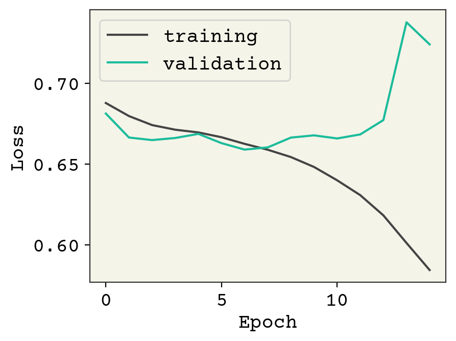
plt.plot(train_losses, label="training")
plt.plot(val_losses, label="validation")
plt.legend()
plt.xlabel("Epoch")
plt.ylabel("Loss")
plt.show()
print("epoch 0", val_accuracies[0], f"epoch {len(val_accuracies)}", val_accuracies[-1])
epoch 0 0.5468834688346883 epoch 15 0.5615176151761517
You can see this is a classic case of overfitting, with the validation data rising quickly as we improve our loss on the training data. Indeed, our model is quite expressive in its capability to fit the training data but it is incidentally fititng the noise. We have 61,000 trainable parameters and about 15,000 training examples, so this is not a surprise. However, we still able to learn a little bit – our accuracy is above 50%. This is actually a challenging dataset and the state-of-the art result is 77% accuracy [KRK+18]. We need to expand our tools to include layers that can address overfitting.
7.5. Back propagation#
At this stage, we should probably talk about back propagation and its connection to automatic gradient computation (autograds). This is how training “just works” when we take a gradient. This is actually a bit of a complicated topic, but it also nearly invisible to users of modern deep learning packages. Thus, I have chosen to not cover it in this book. You can find comprehensive discussions of modern autograd in [BPRS18] and in the Jax manual.
7.6. Regularization#
As we saw in the ML chapters, regularization is a strategy that changes your training procedure (often by adding loss terms) to prevent overfitting. There is a nice argument for it in the bias-variance trade-off regarding model complexity, however this doesn’t seem to hold in practice [NMB+18]. Thus, we view regularization as an empirical process. Regularization, like other hyperparameter tuning, is dependent on the layers, how complex your model is, your data, and especially if your model is underfit or overfit. Underfitting means you could train longer to improve validation loss. Adding regularization if your model is underfit will usually reduce performance. Consider training longer or adjusting learning rates if you observe this.
7.6.1. Early Stopping#
The most commonly used and simplest form of regularization is early stopping. Early stopping means monitoring the loss on your validation data and stopping training once it begins to rise. Normally, training is done until converged – meaning the loss stops decreasing. Early stopping tries to prevent overfitting by looking at the loss on unseen data (validation data) and stopping once that begins to rise. This is an example of regularization because the weights are limited to move a fixed distance from their initial value. Just like in L2 regularization, we’re squeezing our trainable weights. Early stopping can be a bit more complicated to implement in practice than it sounds, so check out how frameworks do it before trying to implement yourself (e.g., tf.keras.callbacks.EarlyStopping).
7.6.2. Weight Decay (regularization)#
Weight regularization is the addition of terms to the loss that depend on the trainable weights in the solubility model example. These can be L2 (\(\sqrt{\sum w_i^2}\)) or L1 (\(\sum \left|w_i\right|\)). You must choose the strength, which is expressed as a parameter (often denoted \(\lambda\)) that should be much less than \(1\). Typically values of \(0.1\) to \(1\times10^{-4}\) are chosen. This may be broken into kernel regularization, which affects the multiplicative weights in a dense or convolution neural network, and bias regularization. Bias regularization is rarely seen in practice.
This is more commonly known as weight decay and implemented in optimizers directly.
7.6.3. Activity#
Activity regularization is the addition of terms to the loss that depend on the output from a layer. Activity regularization ultimately leads to minimizing weight magnitudes, but it makes the strength of that effect depend on the output from the layers. Weight regularization has the strongest effect on weights that have little effect on layer output, because they have no gradient if they have little effect on the output. In contrast, activity regularization has the strongest effect on weights that greatly affect layer output. Conceptually, weight regularization reduces weights that are unimportant but could harm generalization error if there is a shift in the type of features seen in testing. Activity regularization reduces weights that affect layer output and is more akin to early stopping by reducing how far those weights can move in training.
7.6.4. Batch Normalization#
It is arguable if batch normalization is a regularization technique – there is often debate about why it’s effective. Batch normalization is a layer that is added to a neural network with trainable weights [IS15]. Batch normalization has a layer equation of:
where \(\bar{X}\) and \(S\) are the sample mean and variance taken across the batch axis. This has the effect of “smoothing” out the magnitudes of values seen between batches. \(\gamma\) and \(\beta\) are optional trainable parameters that can move the output mean and variance to be \(\beta\) and \(\gamma\), respectively. Remember that activations like ReLU depend on values being near 0 (since the nonlinear part is at \(x = 0\)) and tanh has the most change in output around \(x = 0\), so you typically want your intermediate layer outputs to be around \(0\). But, \(\gamma\) and \(\beta\) allow the optimum output to be learned. At inference time you may not have batches or your batches may be a different size, so \(\bar{X}\) and \(S\) are set to the average across all batches seen in training data. A common explanation of batch normalization is that it smooths out the optimization landscape by forcing layer outputs to be approximately normal[STIMkadry18].
7.6.4.1. Layer Normalization#
Batch normalization depends on there being a constant batch size. Some kinds of data, like text or graphs, have different sizes and so the batch mean/variance can change significantly. Layer normalization avoids this problem by normalizing across the features (the non-batch axis/channel axis) instead of the batch. This has a similar effect of making the layer output features behave well-centered at 0 but without having highly variable means/variances because of batch to batch variation. You’ll see these in graph neural networks and recurrent neural networks, with both take variable sized inputs.
7.6.5. Dropout#
The last regularization type is dropout. Like batch normalization, dropout is typically viewed as a layer and has no trainable parameters. In dropout, we randomly zero-out specific elements of the input and then rescale the output so its average magnitude is unchanged. You can think of it like masking. There is a mask tensor \(M\) which contains 1s and 0s and is multiplied by the input. It is called masking because we mask whatever was in the elements that were multiplied by 0. Then the output is multiplied by \(|M| / \sum M\) where \(|M|\) is the number of elements in \(M\). Dropout forces your neural network to learn to use different features or “pathways” by zeroing out elements. Weight regularization squeezes unused trainable weights through minimization. Dropout tries to force all trainable weights to be used by randomly negating weights. Dropout is more common than weight or activity regularization but has arguable theoretical merit. Some have proposed it is a kind of sampling mechanism for exploring model variations[GG16]. Despite it appearing ad-hoc, it is effective. Note that dropout is only used during training, not for inference. You need to choose the dropout rate when using it, another hyperparameter. Usually, you will want to choose a rate of 0.05–0.35. 0.2 is common. Too small of a value – meaning you rarely do dropout – makes the effect too small to matter. Too large of a value – meaning you often dropout values – can prevent you from actually learning. As fewer nodes get updated with dropout, larger learnings rates with decay and a larger momentum can help with the model’s performance.
Fig. 7.2 Dropout.#
7.7. Residues#
One last “layer” note to mention is residues. One of the classic problems in neural network training is vanishing gradients. If your neural network is deep and many features contribute to the label, you can have very small gradients during training that make it difficult to train. This is visible as underfitting. One way this can be addressed is through careful choice of optimization and learning rates. Another way is to add “residue” connections in the neural network. Residue connections are a fancy way of saying “adding” or “concatenating” later layers with early layers. The most common way to do this is:
This is the usual equation for a dense neural network but we’ve added the previous layer output (\(X^i\)) to our output. Now when you take a gradient of earlier weights from layer \(i - 1\), they will appear through both the \(\sigma(W^iX^i + b^i)\) term via the chain rule and the \(X^i\) term. This goes around the activation \(\sigma\) and the effect of \(W^i\). Note this continues at all layers and then a gradient can propagate back to earlier layers via either term. You can add the “residue” connection to the previous layer as shown here or go back even earlier. You can also be more complex and use a trainable function for how the residue term (\(X^i\)) can be treated. For example:
where \(W'^i\) is a set of new trainable parameters. We have seen that there are many hyperparametes for tuning and adjusting residue connections is one of the least effective things to adjust. So don’t expect much of an improvement. However, if you’re seeing underfitting and inefficient training, perhaps it’s worth investigating.
7.8. Blocks#
You can imagine that we might join a dense layer with dropout, batch normalization, and maybe a residue. When you group multiple layers together, this can be called a block for simplicity. For example, you might use the word “convolution block” to describe a sequential layers of convolution, pooling, and dropout.
7.9. Dropout Regularization Example#
Now let’s try to add a few dropout layers to see if we can do better on our example above.
#---- SAME AS ABOVE -----#
class SolubilityNetDropout(nn.Module):
    def __init__(self):
        super(SolubilityNetDropout, self).__init__()

        self.embedding = nn.Embedding(num_embeddings=21, embedding_dim=2, padding_idx=0)
        self.conv1 = nn.Conv1d(in_channels=2, out_channels=16, kernel_size=5)
        self.pool1 = nn.MaxPool1d(kernel_size=4)
        self.conv2 = nn.Conv1d(in_channels=16, out_channels=16, kernel_size=3)
        self.pool2 = nn.MaxPool1d(kernel_size=2)
        self.conv3 = nn.Conv1d(in_channels=16, out_channels=16, kernel_size=3)
        self.pool3 = nn.MaxPool1d(kernel_size=2)
        self.flatten = nn.Flatten()
        self.fc1 = nn.Linear(160, 256)
        self.fc2 = nn.Linear(256, 64)
        self.fc3 = nn.Linear(64, 1)
        self.relu = nn.ReLU()
        self.sigmoid = nn.Sigmoid()

        #---- START NEW CODE ---#
        self.d1 = nn.Dropout(0.3)
        self.d2 = nn.Dropout(0.3)
        self.d3 = nn.Dropout(0.3)
        #---- END NEW CODE ---#

    def forward(self, x):
        x = self.embedding(x)
        x = x.transpose(1, 2)
        x = self.pool1(self.relu(self.conv1(x)))
        x = self.pool2(self.relu(self.conv2(x)))
        x = self.pool3(self.relu(self.conv3(x)))
        x = self.flatten(x)

        #---- START NEW CODE ---#
        x = self.relu(self.fc1(self.d1(x)))
        x = self.relu(self.fc2(self.d2(x)))
        x = self.sigmoid(self.fc3(self.d3(x)))
        #---- END NEW CODE ---#


        return x

model = SolubilityNetDropout()
print(model)

params = sum(p.numel() for p in model.parameters() if p.requires_grad)

print(f"\nTotal trainable parameters: {params:,}")
SolubilityNetDropout(
  (embedding): Embedding(21, 2, padding_idx=0)
  (conv1): Conv1d(2, 16, kernel_size=(5,), stride=(1,))
  (pool1): MaxPool1d(kernel_size=4, stride=4, padding=0, dilation=1, ceil_mode=False)
  (conv2): Conv1d(16, 16, kernel_size=(3,), stride=(1,))
  (pool2): MaxPool1d(kernel_size=2, stride=2, padding=0, dilation=1, ceil_mode=False)
  (conv3): Conv1d(16, 16, kernel_size=(3,), stride=(1,))
  (pool3): MaxPool1d(kernel_size=2, stride=2, padding=0, dilation=1, ceil_mode=False)
  (flatten): Flatten(start_dim=1, end_dim=-1)
  (fc1): Linear(in_features=160, out_features=256, bias=True)
  (fc2): Linear(in_features=256, out_features=64, bias=True)
  (fc3): Linear(in_features=64, out_features=1, bias=True)
  (relu): ReLU()
  (sigmoid): Sigmoid()
  (d1): Dropout(p=0.3, inplace=False)
  (d2): Dropout(p=0.3, inplace=False)
  (d3): Dropout(p=0.3, inplace=False)
)

Total trainable parameters: 59,515
train_losses, val_losses, train_accuracies, val_accuracies = training_loop(model)
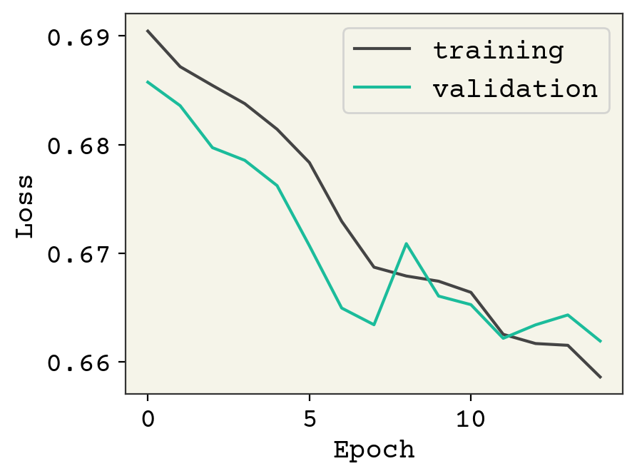
plt.plot(train_losses, label="training")
plt.plot(val_losses, label="validation")
plt.legend()
plt.xlabel("Epoch")
plt.ylabel("Loss")
plt.show()
print("epoch 0", val_accuracies[0], f"epoch {len(val_accuracies)}", val_accuracies[-1])
epoch 0 0.5360433604336043 epoch 15 0.578319783197832
We added a few dropout layers and now we can see the validation loss is a little better but additional training will indeed result it in rising. Feel free to try the other ideas above to see if you can get the validation loss to decrease like the training loss.
7.10. Activation Functions#
Recall in Deep Learning Overview we mentioned that activation functions must be nonlinear and we often want them to have a region of input where the output value is zero. ReLU is the simplest example that satisfies these conditions - its output is zero for negative inputs and \(f(x) = x\) for positive values. Choosing activation is another hyperparameter and choice that we make. People used activations like \(\tanh\) or sigmoids in early neural network research. ReLU began to dominate in modern deep learning because it’s so efficient that models could be made larger for the same runtime speed.

Fig. 7.3 Comparison of the usual ReLU activation function and GELU and Swish.#
Since 2019, this has been revisited because modern GPUs can run a variety of activation functions now quite quickly[EYG19]. Two commonly used modern activation functions are Gaussian Error Linear Units (GELU)[HG16] and Swish[EYG19]. They are shown in Fig. 7.3. They have these two properties of nonlinearity and an ability to turn-off at negative values. They seem to give better results because of their non-zero gradient at negative values; they can continue to respond to gradients while they are turned off. It is more common now to see Swish than ReLU in most newer networks and GELU is specifically seen in transformers (discussed in Deep Learning on Sequences).
The equation for Swish is:
and the equation for GELU is:
7.11. Discussion#
Designing and training neural networks is a complex task. The best approach is to always start simple and work your way up in complexity. Remember, you have to write correct code, create a competent model, and have clean data. If you start with a complex model it can be hard to discern if learning problems are due to bugs, the model, or the data. My advice is to always start with a pre-trained or simple baseline network from a previous paper. If you find yourself designing and training your own neural network, read through Andrej Karpathy’s excellent guide on how to approach this task.
7.12. Chapter Summary#
Layers are created for specific tasks, and given the variety of layers, there are a vast number of permutations of layers in a deep neural network.
Convolution layers are used for data defined on a regular grid (such as images). In a convolution, one defines the size of the trainable parameters through the kernel shape.
An invariance is when the output from a neural network is insensitive to spatial changes in the input (translation, rotation, rearranging order)
An equivariance is when the output from a neural network changes the same way as the input. See Input Data & Equivariances and Equivariant Neural Networks for concrete definitions.
Convolution layers are often paired with pooling layers. A pooling layer behaves similarly to a convolution layer, except a reduction is computed and the output is a smaller shape (same rank) than the input.
Embedding layers convert indices into vectors, and are typically used as pre-processing steps.
Hyperparameters are choices regarding the shape of the layers, the activation function, initialization parameters, and other layer arguments. They can be tuned but are not trained on the data.
Hyperparameters must be tuned by hand, as they can be continuous, categorical, or discrete variables, but there are algorithms being researched that tune hyperparameters.
Tuning the hyperparameters can make training faster or require less training data.
Using a validation data set can measure the overfitting of training data, and is used to help choose the hyperparameters.
Regularization is an empirical technique used to change training procedures to prevent overfitting. There are five common types of regularization: early stopping, weight regularization, activity regularization, batch normalization, and dropout.
Vanishing gradient problems can be addressed by adding “residue” connections, essentially adding later layers with early layers in the neural network.
7.13. Cited References#
Brady Neal, Sarthak Mittal, Aristide Baratin, Vinayak Tantia, Matthew Scicluna, Simon Lacoste-Julien, and Ioannis Mitliagkas. A modern take on the bias-variance tradeoff in neural networks. arXiv preprint arXiv:1810.08591, 2018.
Xavier Glorot and Yoshua Bengio. Understanding the difficulty of training deep feedforward neural networks. In Proceedings of the thirteenth international conference on artificial intelligence and statistics, 249–256. 2010.
Dan Claudiu Cireşan, Ueli Meier, Luca Maria Gambardella, and Jürgen Schmidhuber. Deep, big, simple neural nets for handwritten digit recognition. Neural computation, 22(12):3207–3220, 2010.
Chelsea Finn, Pieter Abbeel, and Sergey Levine. Model-agnostic meta-learning for fast adaptation of deep networks. In International conference on machine learning, 1126–1135. PMLR, 2017.
Barret Zoph and Quoc V. Le. Neural architecture search with reinforcement learning. arXiv preprint arXiv:1611.01578, 2017. URL: https://arxiv.org/abs/1611.01578.
Lisha Li, Kevin Jamieson, Giulia DeSalvo, Afshin Rostamizadeh, and Ameet Talwalkar. Hyperband: a novel bandit-based approach to hyperparameter optimization. Journal of Machine Learning Research, 18(185):1–52, 2018. URL: http://jmlr.org/papers/v18/16-558.html.
Catherine Ching Han Chang, Jiangning Song, Beng Ti Tey, and Ramakrishnan Nagasundara Ramanan. Bioinformatics approaches for improved recombinant protein production in escherichia coli: protein solubility prediction. Briefings in bioinformatics, 15(6):953–962, 2014.
Y. Lecun, L. Bottou, Y. Bengio, and P. Haffner. Gradient-based learning applied to document recognition. Proceedings of the IEEE, 86(11):2278–2324, 1998.
Sameer Khurana, Reda Rawi, Khalid Kunji, Gwo-Yu Chuang, Halima Bensmail, and Raghvendra Mall. DeepSol: a deep learning framework for sequence-based protein solubility prediction. Bioinformatics, 34(15):2605–2613, 03 2018. URL: https://doi.org/10.1093/bioinformatics/bty166, doi:10.1093/bioinformatics/bty166.
Atilim Gunes Baydin, Barak A Pearlmutter, Alexey Andreyevich Radul, and Jeffrey Mark Siskind. Automatic differentiation in machine learning: a survey. Journal of Marchine Learning Research, 18:1–43, 2018.
Sergey Ioffe and Christian Szegedy. Batch normalization: accelerating deep network training by reducing internal covariate shift. In International conference on machine learning, 448–456. PMLR, 2015.
Shibani Santurkar, Dimitris Tsipras, Andrew Ilyas, and Aleksander Mądry. How does batch normalization help optimization? In Proceedings of the 32nd international conference on neural information processing systems, 2488–2498. 2018.
Yarin Gal and Zoubin Ghahramani. Dropout as a bayesian approximation: representing model uncertainty in deep learning. In international conference on machine learning, 1050–1059. 2016.
Steffen Eger, Paul Youssef, and Iryna Gurevych. Is it time to swish? comparing deep learning activation functions across nlp tasks. arXiv preprint arXiv:1901.02671, 2019.
Dan Hendrycks and Kevin Gimpel. Gaussian error linear units (gelus). arXiv preprint arXiv:1606.08415, 2016.