15. Normalizing Flows#
The VAE was our first example of a generative model that is capable of sampling from \(P(x)\). A VAE can also estimate \(P(x)\) by going from the encoder to \(z\), and then using the known distribution \(P(z)\). However, VAEs typically are not great at either tasks. Their samples are often described as “blurry” because they have mean-seeking behavior. That is, the individual samples do not correspond to a very likely example (not mode-seeking). Instead the distribution of samples is good (mean-seeking). Generative adversarial networks (GANs) are an alternative to VAEs which have high probability samples. However, both methods suffer often have training problems and also give poor estimates of \(P(x)\) because of both lack of normalization and assumptions of normal distributions. An alternative is a normalizing flow that has better stability training and better estimates of \(P(x)\). Normalizing flows are also used as components in other networks, like it can act as \(P(z)\) of a latent space for a VAE instead of standard normal distributions.
A normalizing flow is similar to a VAE in that we try to build up \(P(x)\) by starting from a simple known distribution \(P(z)\). We use functions, like the decoder from a VAE, to go from \(x\) to \(z\). However, we make sure that the functions we choose keep the probability mass normalized (\(\sum P(x) = 1\)) and can be used forward (to sample from x) and backward (to compute \(P(x)\)). We call these functions bijectors because they are bijective (surjective and injective). Recall surjective (onto) means every output has a corresponding input and injective (onto) means each output has exactly one corresponding input.
An example of a bijector is an element-wise cosine \(y_i = \cos x_i\) (assuming \(x_i\) is between \(0\) and \(\pi\)). A non-bijective function would be \(y_i = \cos x_i\) on the interval from \(0\) to \(2\pi\), because it outputs all values from \([0,1]\) twice and hence is not injective. Any function which changes the number of elements is automatically not bijective (see margin note). A consequence of using only bijectors in constructing our normalizing flow is that the size of the latent space must be equal to the size of the feature space. Remember the VAE used a smaller latent space than the feature space.
Audience & Objectives
This chapter builds on Variational Autoencoder and assumes the same background of probability theory. This chapter is an introduction to the key ideas, but is not fully developed yet. Some knowledge of vector calculus (Jacobians) is assumed as well. After completing it, you should be able to
Understand the trade-offs between a VAE, GAN, and normalizing flow.
Identify a bijector and construct a bijector chain
Construct a normalizing flow using common bijectors types and train it
Sample from a normalizing flow and compute sample probabilities
You can find a recent review of normalizing flows here [KPB20] and here[PNR+19]. Although generating images and sound is the most popular application of normalizing flows, some of their biggest scientific impact has been on more efficient sampling from posteriors or likelihoods and other complex probability distributions [PSM19]. You find details on how to do normalizing flows on categorical (discrete) data in Hoogeboom et al. [HNJ+21].
15.1. Flow Equation#
Recall for the VAE decoder, we had an explicit formula for \(p(x | z)\). This allowed us to compute \(p(x) = \int\,dz p(x | z)p(z)\) which is the quantity of interest. The VAE decoder is a conditional probability density function. In the normalizing flow, we do not use probability density functions. We use bijective functions. So we cannot just compute an integral to change variables. We can use the change of variable formula. Consider our normalizing flow to be defined by our bijector \(x = f(z)\), its inverse \(z = g(x)\), and the starting probability distribution \(P_z(z)\). Then the formula for probability of \(x\) is
where the term on the right is the absolute value of the determinant of the Jacobian of \(g\). Jacobians are matrices that describe how infinitesimal changes in each domain dimension change each range dimension. This term corrects for the volume change of the distribution. For example, if \(f(z) = 2z\), then \(g(x) = x / 2\), and the Jacobian determinant is \(1 / 2\). The intuition is that we are stretching out \(z\) by 2, so we need to account for the increase in volume to keep the probability normalized. You can read more about the change of variable formula for probability distributions here
15.2. Bijectors#
A bijector is a function that is injective (1 to 1) and surjective (onto). An equivalent way to view a bijective function is if it has an inverse. For example, a sum reduction has no inverse and is thus not bijective. \(\sum [1,0] = 1\) and \(\sum [-1, 2] = 1\). Multiplying by a matrix which has an inverse is bijective. \(y = x^2\) is not bijective, since \(y = 4\) has two solutions.
Remember that we must compute the determinant of the bijector Jacobian. If the Jacobian is dense (all output elements depend on all input elements), computing this quantity will be \(O\left(|x|_0^3\right)\) where \(|x|_0\) is the number of dimensions of \(x\) because a determinant scales by \(O(n^3)\). This would make computing normalizing flows impractical in high-dimensions. However, in practice we restrict ourselves to bijectors that have easy to calculate Jacobians. For example, if the bijector is \(x_i = \cos z_i\) then the Jacobian will be diagonal. Such a diagonal Jacobian means that each dimension is independent of the other though.
One way to get faster determinants without just making each dimension independent is to get a triangular Jacobian. Then \(x_0\) only depends on \(z_0\), \(x_1\) depends on \(z_0, z_1\), and \(x_2\) depends on \(z_0, z_1, z_2\), etc. This enables fitting high-dimensional correlations for some of the dimensions (like \(x_{n}\)). The matrix determinant of a triangular matrix is computed in linear time with respect to the number of dimensions – because it is just the product of the matrix diagonal.
15.2.1. Bijector Chains#
Just like in deep neural networks, multiple bijectors are chained together to increase how complex of the final fit distribution \(\hat{P}(x)\) can be. The change of variable equation can be repeatedly applied:
where we would compute \(x\) with \(f_0\left(f_1(z)\right)\). One critical point is that you should also include a permute bijector that swaps the order of dimensions. Since the bijectors typically have triangular Jacobians, certain output dimensions will depend on many input dimensions and others will only depend on a single one. By applying a permutation, you allow each dimension to influence each other.
15.3. Training#
At this point, you may be wondering how you could possibly train a normalizing flow. The trainable parameters appear in the bijectors. They have adjustable parameters. The loss equation is quite simple: the negative log-likelihood (negative to make it minimization). Explicitly:
where \(x\) is the training point and when you take the gradient of the loss, it is with respect to the parameters of the bijectors.
15.4. Common Bijectors#
The choice of bijector functions is a fast changing area. I will thus only mention a few. You can of course use any bijective function or matrix, but these become inefficient at high-dimension due to the Jacobian calculation. One class of efficient bijectors are autoregressive bijectors. These have triangular Jacobians because each output dimension can only depend on the dimensions with a lower index. There are two variants: masked autoregressive flows (MAF)[PPM17] and inverse autoregressive flows (IAF) [KSJ+16]. MAFs are efficient at training and computing probabilities, but are slow for sampling from \(P(x)\). IAFs are slow at training and computing probabilities but efficient for sampling. Wavenets combine the advantages of both [KLS+18]. I’ll mention one other common bijector which is not autoregressive: real non-volume preserving (RealNVPs) [DSDB16]. RealNVPs are less expressive than IAFs/MAFs, meaning they have trouble replicating complex distributions, but are efficient at all three tasks: training, sampling, and computing probabilities. Another interesting variant is the Glow bijector,which is able to expand the rank of the normalizing flow, for example going from a matrix to an RGB image [DAS19]. What are the equations for all these bijectors? Most are variants of standard neural network layers but with special rules about which outputs depend on which inputs.
Warning
Remember to add permute bijectors between autoregressive bijectors to ensure the dependence between dimensions is well-mixed.
15.5. Running This Notebook#
Click the above to launch this page as an interactive Google Colab. See details below on installing packages.
Tip
To install packages, execute this code in a new cell.
!pip install dmol-book
If you find install problems, you can get the latest working versions of packages used in this book here
The hidden code below imports the normflows package and other necessary packages. The normflows package provides distributions, bijective flows, and normalizing flow models.
import torch
import normflows as nf
import matplotlib.pyplot as plt
import sklearn.datasets as datasets
import numpy as np
import dmol
np.random.seed(0)
torch.manual_seed(0)
<torch._C.Generator at 0x7f93b82e8690>
15.6. Moon Example#
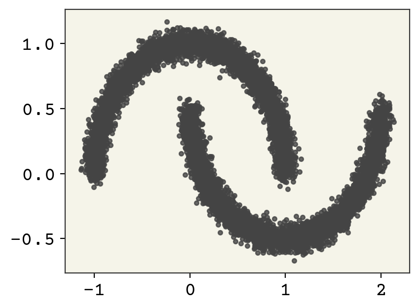
We’ll start with a basic 2D example to learn the two moons distribution with a normalizing flow. Two moons is a common example dataset that is hard to cluster and model as a probability distribution.
When doing normalizing flows you have two options to implement them. You can do all the Jacobians, inverses, and likelihood calculations analytically and implement them in a normal ML framework like Jax, PyTorch, or TensorFlow. This is actually most common. The second option is to utilize a probability library that knows how to use bijectors and distributions. We’ll use normflows, a PyTorch-based library for normalizing flows.
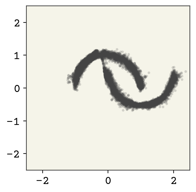
15.6.1. Generating Data#
In the code below, I set-up my imports and sample points which will be used for training. Remember, this code has nothing to do with normalizing flows – it’s just to generate data.
moon_n = 10000
ndim = 2
data, _ = datasets.make_moons(moon_n, noise=0.05)
plt.plot(data[:, 0], data[:, 1], ".", alpha=0.8)
[<matplotlib.lines.Line2D at 0x7f925bb14cd0>]
15.6.2. Z Distribution#
Our Z distribution should always be as simple as possible. I’ll create a 2D Gaussian with unit variance, no covariance, and centered at 0. We’ll use the normflows package, which provides distributions, flows (bijectors), and the normalizing flow model class that handles change of variable calculations automatically.
zdist = nf.distributions.DiagGaussian(ndim)
zdist
DiagGaussian()
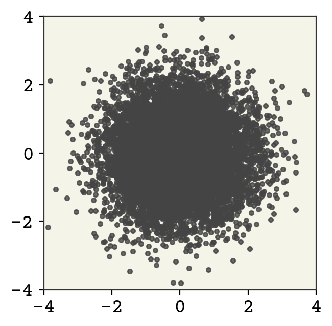
This is a 2D diagonal Gaussian. Let’s now sample from this distribution and view it.
zsamples = zdist.sample(moon_n).detach().numpy()
plt.plot(zsamples[:, 0], zsamples[:, 1], ".", alpha=0.8)
plt.xlim(-4, 4)
plt.ylim(-4, 4)
plt.gca().set_aspect("equal")
As expected, our starting distribution looks nothing like are target distribution. Let’s demonstrate a bijector now. We’ll implement the following bijector:
This is bijective because the operations are element-wise and invertible. We’ll use the Affine flow from normflows, which implements \(x = s \odot z + t\) where \(s\) is a scale and \(t\) is a shift.
b = nf.flows.AffineConstFlow((ndim,))
b.s.data = torch.log(torch.tensor([[1.0, 0.5]]))
b.t.data = torch.tensor([[0.5, 0.25]])
To now apply the change of variable formula, we create a normalizing flow model. What is important about this is that we can compute log-likelihoods and sample from it.
td = nf.NormalizingFlow(zdist, [b])
td
NormalizingFlow(
  (q0): DiagGaussian()
  (flows): ModuleList(
    (0): AffineConstFlow()
  )
)
zsamples = td.sample(moon_n)[0].detach().numpy()
plt.plot(zsamples[:, 0], zsamples[:, 1], ".", alpha=0.8)
plt.xlim(-4, 4)
plt.ylim(-4, 4)
plt.gca().set_aspect("equal")
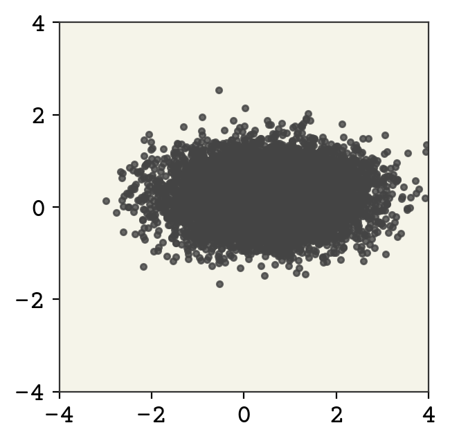
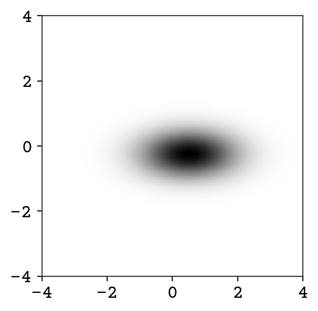
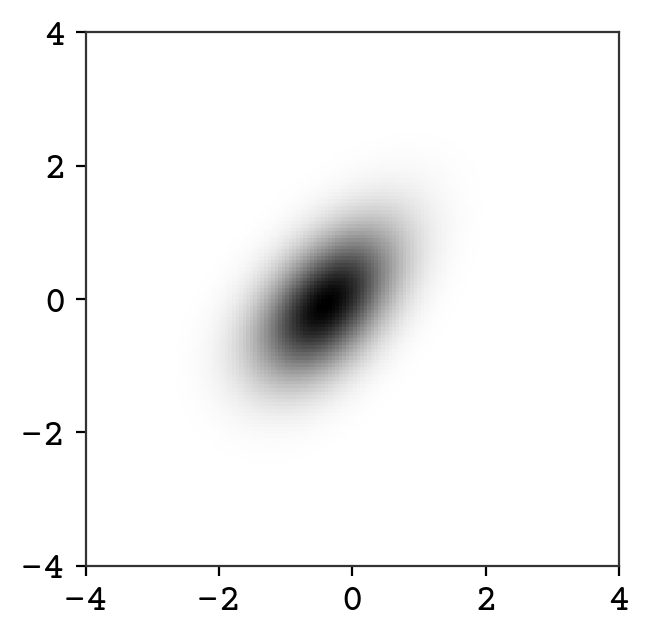
We show above the sampling from this new distribution. We can also plot it’s probability, which is impossible for a VAE-like model!
# make points for grid
zpoints = np.linspace(-4, 4, 150)
(
    z1,
    z2,
) = np.meshgrid(zpoints, zpoints)
zgrid = np.concatenate((z1.reshape(-1, 1), z2.reshape(-1, 1)), axis=1)
# compute P(x)
p = np.exp(td.log_prob(torch.tensor(zgrid, dtype=torch.float32)).detach().numpy())
fig = plt.figure()
# plot and set axes limits
plt.imshow(p.reshape(z1.shape), aspect="equal", extent=[-4, 4, -4, 4])
plt.show()
15.6.3. The Normalizing Flow#
Now we will build bijectors that are expressive enough to capture the moon distribution. I will use 3 sets of a MAF and permutation for 6 total bijectors. MAF’s have dense neural network layers in them, so I will also set the usual parameters for a neural network: dimension of hidden layer and activation.
Note
It may seem counterintuitive that we use ReLU activation functions, which are not bijective, inside a bijector. The reason this works is that the neural network (which uses ReLU) is used to output the parameters (scale and shift) of the affine transformation. The transformation itself is \(y = x \odot \exp(s) + t\), which is bijective regardless of how \(s\) and \(t\) are computed (as long as they are deterministic functions of the input).
num_layers = 3
my_flows = []
for i in range(num_layers):
    my_flows.append(nf.flows.MaskedAffineAutoregressive(ndim, 128, 2))
    my_flows.append(nf.flows.LULinearPermute(ndim))

base = nf.distributions.DiagGaussian(ndim)
td = nf.NormalizingFlow(base, my_flows)
At this point, we have not actually trained but we can still view our distribution.
zpoints = np.linspace(-4, 4, 150)
(
    z1,
    z2,
) = np.meshgrid(zpoints, zpoints)
zgrid = np.concatenate((z1.reshape(-1, 1), z2.reshape(-1, 1)), axis=1)
p = np.exp(td.log_prob(torch.tensor(zgrid, dtype=torch.float32)).detach().numpy())
fig = plt.figure()
plt.imshow(p.reshape(z1.shape), aspect="equal", extent=[-4, 4, -4, 4])
plt.show()
You can already see that the distribution looks more complex than a Gaussian.
15.6.4. Training#
To train, we minimize the negative log-likelihood using PyTorch’s optimizer. The forward_kld method computes the forward KL divergence, which is equivalent to negative log-likelihood on the training data.
optimizer = torch.optim.Adam(td.parameters(), lr=1e-3)
We train by computing the forward KL divergence on mini-batches of our training data.
data_t = torch.tensor(data, dtype=torch.float32)
losses = []
batch_size = 256
epochs = 100
for epoch in range(epochs):
    perm = torch.randperm(moon_n)
    epoch_loss = 0
    for i in range(0, moon_n, batch_size):
        batch = data_t[perm[i : i + batch_size]]
        optimizer.zero_grad()
        loss = td.forward_kld(batch)
        loss.backward()
        optimizer.step()
        epoch_loss += loss.item()
    losses.append(epoch_loss / (moon_n // batch_size))
plt.plot(losses)
plt.show()
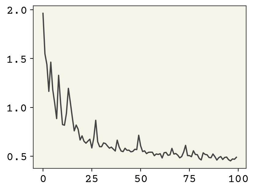
Training looks reasonable. Let’s now see our distribution.
zpoints = np.linspace(-2.5, 2.5, 200)
(
    z1,
    z2,
) = np.meshgrid(zpoints, zpoints)
zgrid = np.concatenate((z1.reshape(-1, 1), z2.reshape(-1, 1)), axis=1)
p = np.exp(td.log_prob(torch.tensor(zgrid, dtype=torch.float32)).detach().numpy())
fig = plt.figure()
plt.imshow(
    p.reshape(z1.shape), aspect="equal", origin="lower", extent=[-2.5, 2.5, -2.5, 2.5]
)
plt.show()
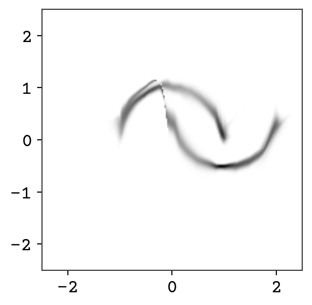
Wow! We now can compute the probability of any point in this distribution. You can see there are some oddities that could be fixed with further training. One issue that cannot be overcome is the connection between the two curves – it is not possible to get fully disconnected densities. This is because of our requirement that the bijectors are invertible and volume preserving – you can only squeeze volume so far but cannot completely disconnect. Some work has been done on addressing this issue by adding sampling to the flow and this gives more expressive normalizing flows [WKohlerNoe20].
Finally, we’ll sample from our model just to show that indeed it is generative.
zsamples = td.sample(moon_n)[0].detach().numpy()
plt.plot(zsamples[:, 0], zsamples[:, 1], ".", alpha=0.2, markeredgewidth=0.0)
plt.xlim(-2.5, 2.5)
plt.ylim(-2.5, 2.5)
plt.gca().set_aspect("equal")
15.7. Relevant Videos#
15.7.1. Normalizing Flow for Molecular Conformation#
15.8. Chapter Summary#
A normalizing flow builds up a probability distribution of \(x\) by starting from a known distribution on \(z\). Bijective functions are used to go from \(z\) to \(x\).
Bijectors are functions that keep the probability mass normalized and are used to go forward and backward (because they have well-defined inverses).
To find the probability distribution of \(x\) we use the change of variable formula, which requires a function inverse and Jacobian.
The bijector function has trainable parameters, which can be trained using a negative log-likelihood function.
Multiple bijectors can be chained together, but typically must include a permute bijector to swap the order of dimensions.
15.9. Cited References#
Ivan Kobyzev, Simon Prince, and Marcus Brubaker. Normalizing flows: an introduction and review of current methods. IEEE Transactions on Pattern Analysis and Machine Intelligence, 2020.
George Papamakarios, Eric Nalisnick, Danilo Jimenez Rezende, Shakir Mohamed, and Balaji Lakshminarayanan. Normalizing flows for probabilistic modeling and inference. arXiv preprint arXiv:1912.02762, 2019.
George Papamakarios, David Sterratt, and Iain Murray. Sequential neural likelihood: fast likelihood-free inference with autoregressive flows. In The 22nd International Conference on Artificial Intelligence and Statistics, 837–848. PMLR, 2019.
Emiel Hoogeboom, Didrik Nielsen, Priyank Jaini, Patrick Forré, and Max Welling. Argmax flows: learning categorical distributions with normalizing flows. In Third Symposium on Advances in Approximate Bayesian Inference. 2021. URL: https://openreview.net/forum?id=fdsXhAy5Cp.
George Papamakarios, Theo Pavlakou, and Iain Murray. Masked autoregressive flow for density estimation. In Advances in Neural Information Processing Systems, 2338–2347. 2017.
Durk P Kingma, Tim Salimans, Rafal Jozefowicz, Xi Chen, Ilya Sutskever, and Max Welling. Improved variational inference with inverse autoregressive flow. In Advances in neural information processing systems, 4743–4751. 2016.
Sungwon Kim, Sang-gil Lee, Jongyoon Song, Jaehyeon Kim, and Sungroh Yoon. Flowavenet: a generative flow for raw audio. arXiv preprint arXiv:1811.02155, 2018.
Laurent Dinh, Jascha Sohl-Dickstein, and Samy Bengio. Density estimation using real nvp. arXiv preprint arXiv:1605.08803, 2016.
Hari Prasanna Das, Pieter Abbeel, and Costas J Spanos. Dimensionality reduction flows. arXiv preprint arXiv:1908.01686, 2019.
Hao Wu, Jonas Köhler, and Frank Noé. Stochastic normalizing flows. arXiv preprint arXiv:2002.06707, 2020.