19. Equivariant Neural Network for Predicting Trajectories#
Audience & Objectives
This chapter builds on Equivariant Neural Networks and Input Data & Equivariances. After completing this chapter, you should be able to
Understand the importance of equivariance and how to check for equivariances in your model
Understand how an equivariant model can be implemented in E3NN
Be able to recognize and use the irrep notation used in E3NN
In this example, we will train an equivariant neural network to predict the next frame in the trajectory alignment example in Input Data & Equivariances. As stated in Input Data & Equivariances, for time-dependent trajectories, we do not need to concern ourselves with permutation equivariance because it is implied that the order of the points does not change. Thus, we can treat this example as point cloud, meaning that any deep learning model that we train on this data should have rotation and translation equivariance. In other words, our model should be E(3) equivariant. E3NN is a library built to create equivariant neural networks for the this group, so it’s a great choice for this problem [GS22]. We will look at E3NN in more detail later in the chapter.
19.1. Running This Notebook#
Click the above to launch this page as an interactive Google Colab. See details below on installing packages.
Tip
To install packages, execute this code in a new cell.
!pip install dmol-book
If you find install problems, you can get the latest working versions of packages used in this book here
# additional imports
import torch
import torch_geometric
import e3nn
import matplotlib.pyplot as plt
import urllib.request
import numpy as np
import jax
import dmol
/opt/hostedtoolcache/Python/3.13.11/x64/lib/python3.13/site-packages/tqdm/auto.py:21: TqdmWarning: IProgress not found. Please update jupyter and ipywidgets. See https://ipywidgets.readthedocs.io/en/stable/user_install.html
  from .autonotebook import tqdm as notebook_tqdm
19.2. Retrieving Data from Trajectory Alignment Example#
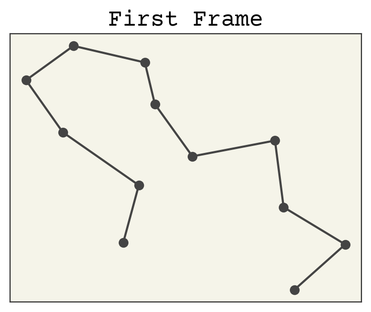
First, let’s borrow a cell from Input Data & Equivariances to download our data and view the first frame.
urllib.request.urlretrieve(
    "https://github.com/whitead/dmol-book/raw/main/data/paths.npz", "paths.npz"
)
paths = np.load("paths.npz")["arr"]
# plot the first point
plt.title("First Frame")
plt.plot(paths[0, :, 0], paths[0, :, 1], "o-")
plt.xticks([])
plt.yticks([])
plt.show()
19.3. Baseline Model#
Before we build our E3NN network, it’s always a good idea to build a baseline model for comparision.
First, let’s discuss what the input and output should be for this model. The input should be the coordinates of the 12 points: one frame. What should the output be? We want to train a neural network to predict the next trajectory for each point, the next frame, so our output should actually be the same type and size as our input.
Thus,
Inputs: 12 sets of coordinates
Outputs: 12 sets of coordinates
Note: since we are trying to build an E(3)-equivariant neural network, which should be equivariant to transformations in 3D space, we need to make these coordinates 3D. This is easy, we will just put zero for the z-coordiantes. We’ll do this now.
traj_3d = np.array([])
for i in range(2048):
    for j in range(12):
        TBA = paths[i][j]
        TBA = np.append(TBA, np.array([0.00]))
        traj_3d = np.append(traj_3d, TBA)

traj_3d = traj_3d.reshape(2048, 12, 3)
Interestingly, for this example, we want our prediction from one frame to match the following frame. So our features and labels will be nearly identical, offset by one. For the features, we want to include everything except for the final frame, which has no “next frame” in our data. We can extrapolate with our model to predict this “next frame” as a final step if we want. For our labels, we want to include everything except for the first step, which is not the “next frame” of anything in our data. We can also go ahead and split our data into training and testing sets. Let’s do an 80:20 split here. We want to make sure not to shuffle our data, as we are predicting order-sensitive data.
features = traj_3d[:-1]
labels = traj_3d[1:]

# split data 80:20
training_set = features[:1637]
training_labels = labels[:1637]
valid_set = features[1637:]
valid_labels = labels[1637:]
Let’s check to make sure our data matches up. Frame 2 in the features set should be the same as Frame 1 in the labels set.
def mse(y, yhat):
    return np.mean((yhat - y) ** 2)
if mse(features[1], labels[0]) == 0:
    print("success! they match!")
else:
    print(mse(features[1], labels[0]))

fig, axs = plt.subplots(ncols=2, squeeze=True, figsize=(16, 4))

axs[0].set_title("Trajectory 1 end")
axs[1].set_title("Trajectory 2 beginning")

for i in range(0, 1, 16):
    axs[0].plot(features[i, :, 0], features[i, :, 1], ".-", alpha=0.2)
    axs[1].plot(labels[i, :, 0], labels[i, :, 1], ".-", alpha=0.2)
for i in range(2):
    axs[i].set_xticks([])
    axs[i].set_yticks([])
success! they match!
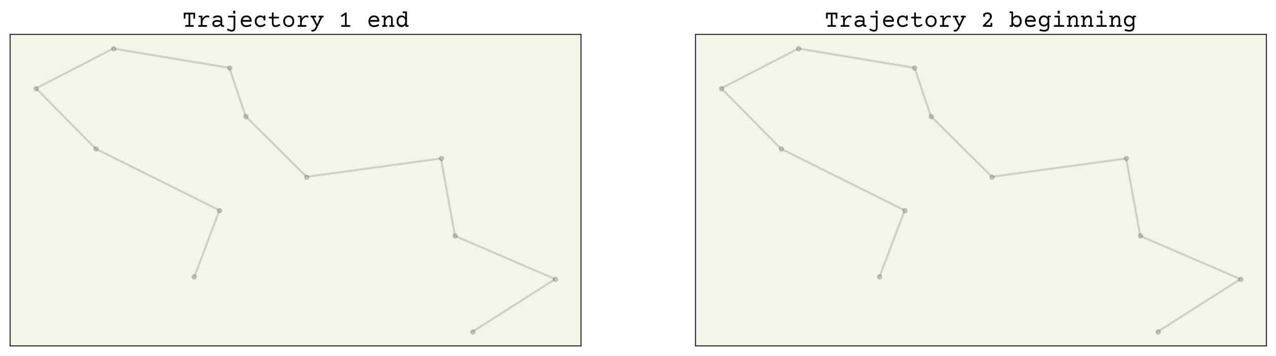
Great, they match! Now we are ready to build our baseline model!
@jax.jit
def baseline_model(inputs, w, b):
    yhat = inputs @ w + b
    return yhat


def baseline_loss(inputs, y, w, b):
    return mse(y, baseline_model(inputs, w, b))


bl_loss_grad = jax.grad(baseline_loss, (2, 3))

w = np.zeros((3, 3))
b = 0.0
epochs = 12
eta = 1e-6

baseline_val_loss = [0.0 for _ in range(epochs)]
ys = []
yhats = []
yst = []
yhatst = []
e = 0

for epoch in range(epochs):
    e += 1
    for d in range(1637):
        inputs = training_set[d]
        y = training_labels[d]
        if e == epochs:
            yhatst.append(baseline_model(inputs, w, b))
            yst.append(y)
        grad_bl = bl_loss_grad(inputs, y, w, b)
        # update w & b
        w -= eta * grad_bl[0]
        b -= eta * grad_bl[1]

    for i in range(410):
        inputs_v = valid_set[i]
        y_v = valid_labels[i]
        if e == epochs:
            yhats.append(baseline_model(inputs_v, w, b))
            ys.append(y_v)
        baseline_val_loss[epoch] += baseline_loss(inputs_v, y_v, w, b)
    baseline_val_loss[epoch] = np.sqrt(baseline_val_loss[epoch] / 410)


plt.plot(baseline_val_loss)
plt.xlabel("Epoch")
plt.ylabel("Val Loss")
plt.show()
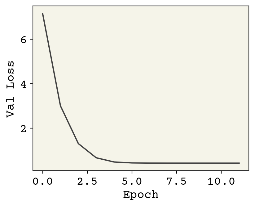
print("Final loss value: ", baseline_val_loss[-1])
Final loss value: 0.43028477
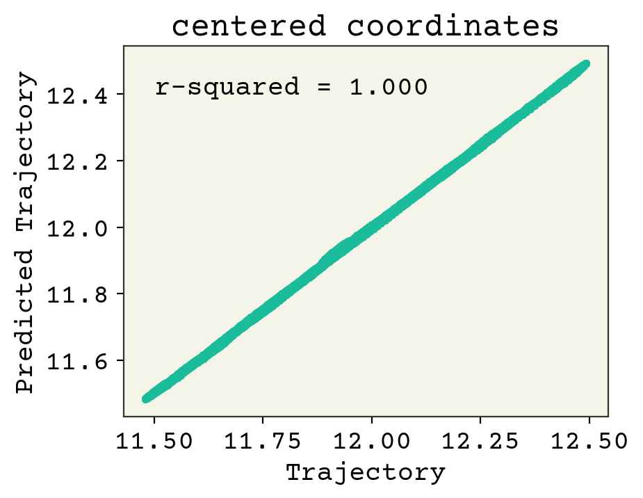
Now let’s view a parity plot to see if we’re learning the right trend here. Since the coordinates are so different in magnitude, we’ll look at a parity plot for the center of mass for each point.
def centerofmass(arr):
    com = []
    for i in arr:
        for j in i:
            avg1 = (j[0] + j[1] + j[2]) / 3
            com.append(avg1)
    return com
from sklearn.metrics import r2_score

y_s = np.stack(ys, axis=0)
yhat_s = np.stack(yhats, axis=0)

ys_centered = centerofmass(y_s)
yhats_centered = centerofmass(yhat_s)

plt.title("centered coordinates")
plt.plot(ys_centered, ys_centered, "-")
plt.plot(ys_centered, yhats_centered, ".")
plt.xlabel("Trajectory")
plt.ylabel("Predicted Trajectory")
plt.annotate(
    "r-squared = {:.3f}".format(r2_score(ys_centered, yhats_centered)), (11.5, 12.4)
)
plt.show()
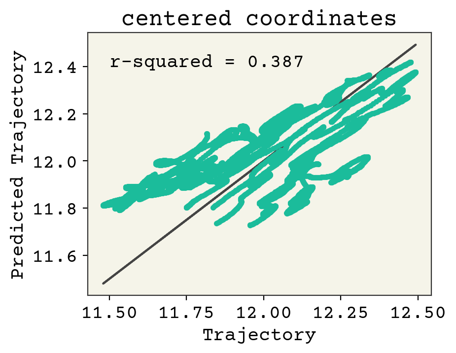
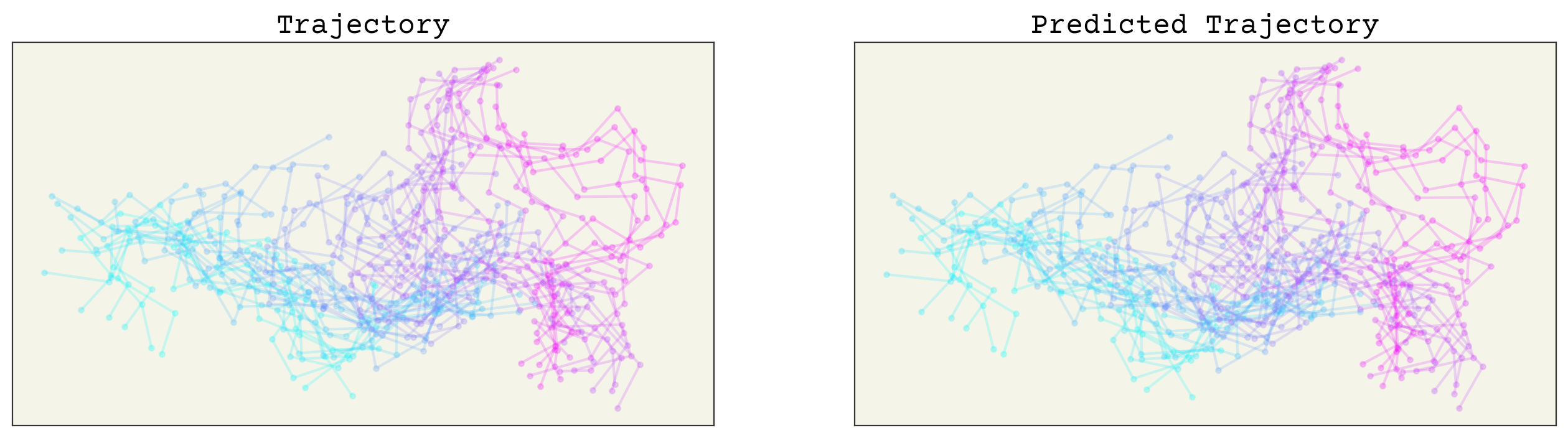
It looks like we are starting to get the right trend for some of the coordinates, but more training is definitely needed. Let’s look at the trajectory labels versus the predicted trajectories. To get a full picture, let’s look add the training and validation data together here.
fig, axs = plt.subplots(ncols=2, squeeze=True, figsize=(16, 4))

y_st = np.stack(yst, axis=0)
ys_total = np.concatenate([y_st, y_s])
yhat_st = np.stack(yhatst, axis=0)
yhats_total = np.concatenate([yhat_st, yhat_s])

axs[0].set_title("Trajectory")
axs[1].set_title("Predicted Trajectory")

cmap = plt.get_cmap("cool")
for i in range(0, 2047, 40):
    axs[0].plot(
        ys_total[i, :, 0], ys_total[i, :, 1], ".-", alpha=0.2, color=cmap(i / 2047)
    )
    axs[1].plot(
        yhats_total[i, :, 0],
        yhats_total[i, :, 1],
        ".-",
        alpha=0.2,
        color=cmap(i / 2047),
    )
for i in range(2):
    axs[i].set_xticks([])
    axs[i].set_yticks([])
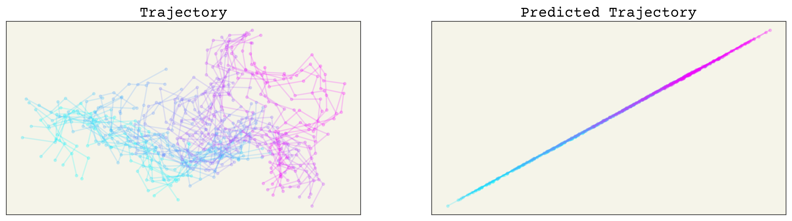
Yikes. Our model does not predict trajectories quite right. We expect this, since our baseline is simple machine learning. Importantly, as stated, we want any model that uses this data to be equivariant in 3D space. Let’s check the equivariances now.
# checking for rotation equivariance
import scipy.spatial.transform as trans

# rotate around x coordinate by 80 degrees
rot = trans.Rotation.from_euler("x", 80, degrees=True)
key = jax.random.PRNGKey(52)

input_point = jax.random.normal(key, (12, 3))
w_test1 = jax.random.normal(key, (3, 3))

input_rot = rot.apply(input_point)
output_1 = baseline_model(input_rot, w_test1, b)
output_prerot = baseline_model(input_point, w_test1, b)
output_rot = []
for xyz in output_prerot:
    coord = rot.apply(xyz)
    output_rot.append(coord)
output_rot = np.asarray(output_rot)


print("\033[1m" + "difference: " + "\033[0m", mse(output_1, output_rot))
fig, axs = plt.subplots(ncols=2, squeeze=True, figsize=(16, 4))
axs[0].set_title("Rotated First")
axs[1].set_title("Rotated Last")

for i in range(0, 1, 16):
    axs[0].plot(output_1[:, 0], output_1[:, 1], ".-", alpha=0.2)
    axs[1].plot(output_rot[:, 0], output_rot[:, 1], ".-", alpha=0.2)
for i in range(2):
    axs[i].set_xticks([])
    axs[i].set_yticks([])
difference: 4.6420107
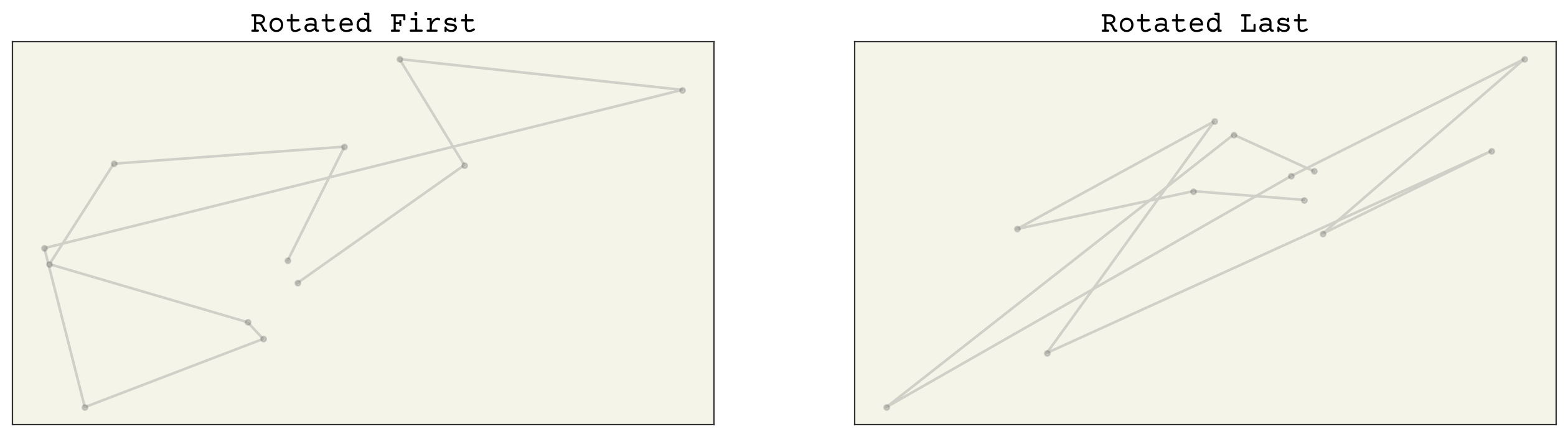
So it doesn’t look like our baseline model is rotation-equivariant. This is important, because if we give our model coordinates that are rotated, we expect the output should be rotated by the same degree. Likewise, we need translation equivariance. Let’s check that now.
# checking for translation equivariance
key2 = jax.random.PRNGKey(9)

random_trans = jax.random.normal(key2, (12, 3))

input_trans = input_point + random_trans
output_2 = baseline_model(input_trans, w_test1, b)
output_trans = random_trans + baseline_model(input_point, w_test1, b)

print("\033[1m" + "difference: " + "\033[0m", mse(output_2, output_trans))
fig, axs = plt.subplots(ncols=2, squeeze=True, figsize=(16, 4))
axs[0].set_title("Translated First")
axs[1].set_title("Translated Last")

for i in range(0, 1, 16):
    axs[0].plot(output_2[:, 0], output_2[:, 1], ".-", alpha=0.2)
    axs[1].plot(output_trans[:, 0], output_trans[:, 1], ".-", alpha=0.2)
for i in range(2):
    axs[i].set_xticks([])
    axs[i].set_yticks([])
difference: 2.1588662
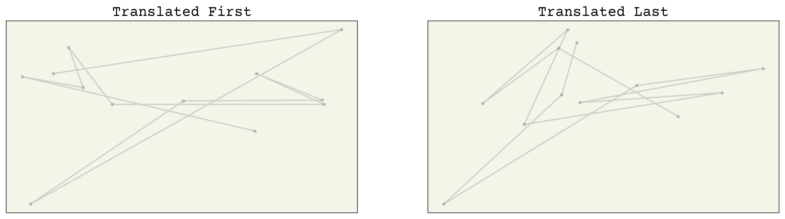
As expected, our model isn’t translation equviariant either. We can solve this problem a few ways. One way is to augment our data in order to teach our model equivariance. This requires more training and data storage, so let’s look at a more compact approach.
19.4. E3NN Basics#
E3NN is a library for creating equivariant neural networks, specifically in E(3). E3NN is built for spatial equvariance in 3-D space, giving us equivariance with respect to the E(3) group of rotations, inversions, and translations. As discussed before, the time-dependent trajectory points do not change order, so we do not need to worry about permutation equivariance/invariance in this case; we only need E(3)-equivariance. E3NN is a great tool for this problem because we have 3-dimensional points in space, and if we transform them in space, we want the output to transform the same way.
E3NN works through the use of irreducible representations (irreps). In general, representations tell you how to interact with the data with repect to the group, and irreducible representations are the smallest and complete representations. When creating a model, we give the model the irreps so that it knows how to handle the data we will give it during trianing. It’s not necessary to understand what the irreps are; instead, just know that they are the smallest representations, which are similar to, and transform the same way as, the spherical harmonics. If you do want more information, you can read about irreps here. Any (reducible) representation can be decomposed into irreducible representations. If you want to know more, you can check out more on the E3NN documentation website [@e3nn]. Let’s take a look at how the irreps are used in this context.
For this group (O(3), which includes parity), we need to find the L and d for each piece of data, where \(d = 2L + 1\) (d = dimension). Look at the table below.
parity |
L |
d |
name |
|---|---|---|---|
even |
0 |
1 |
scalar |
odd |
0 |
1 |
pseudo scalar |
even |
1 |
3 |
pseudo vector |
odd |
1 |
3 |
vector |
even |
2 |
5 |
- |
odd |
2 |
5 |
- |
The general notation is MxLp, where M is the number of 3-D coordinate per input, L is the L (spherical harmonic) from the table above, and p corresponds to the parity (e: even, o: odd).
For example, if you wanted to portray “12 scalars, 4 vectors” in this format, you would write 12x0e + 4x1o. Take a minute to make sure you understand how to use this notation, as it’s essential for E3NN. E3NN deals with equivariance by receiving the irreps as a model parameter. This allows the E3NN framework to know how each input feature/output transforms under symmetry, so that it can treat each piece appropriately. As a side note, the output of an E3NN model must always be of equal or higher symmetry than your input.
Because E3NN is built to handle 3D spatial data, we do not need to tell the model that we are going to give it 3D coordinates; it’s implicit and required. The irreps_in, instead, correspond to the input node features. In this example, we don’t have input features, but as an example, you can imagine we could want our model to predict the next set of coordinates, given the intitial coordinates and the corresponding atom types. In that case, our irreps_in would be the atom types (one scalar per input if we have one-hot vectors).
Since we don’t have input features, we’ll put “None” for that parameter, and we want our output to be the same shape as the input: 12 vectors. However, since we are trying to predict 12 vectors out for 12 vectors in, we only need to tell the model to predict 1 vector per input 1x1o. Take a minute to make sure you understand why this is the case. You can think of the model recognizing 12 input vectors and predicting a vector for each. Again, E3NN expects coordinate inputs, so we don’t specify this for the input.
19.5. E3NN Model#
E3NN has several models within their library, which can be found on the E3NN github page here. For this example, we will use one of these models.
To use the E3NN model, we need to turn our data into a torch_geometric dataset. We’ll do that now. Then we can split our data into training and testing sets.
Also, instead of directly computing the next frame, we’ll change it here to predict the distance to the next frame. This is a small change, but having data centered nearer zero can be better for training. We’ll need to undo this when we look at the frames later.
feat = torch.from_numpy(features)  # convert to pytorch tensors
ys = torch.from_numpy(labels)  # convert to pytorch tensors
traj_data = []
distances = ys - feat  # compute distances to next frame


# make torch_geometric dataset
# we want this to be an iterable list
# x = None because we have no input features
for frame, label in zip(feat, distances):
    traj_data += [
        torch_geometric.data.Data(
            x=None, pos=frame.to(torch.float32), y=label.to(torch.float32)
        )
    ]

train_split = 1637
train_loader = torch_geometric.loader.DataLoader(
    traj_data[:train_split], batch_size=1, shuffle=False
)

test_loader = torch_geometric.loader.DataLoader(
    traj_data[train_split:], batch_size=1, shuffle=False
)
Great! Now we’re ready to define our model. Since this is a pre-built model in E3NN, so we just need to import it and define the model parameters. Note that the state of this model will save automatically, so you will need to reinitialize the model every time you want to start training. To see how these models work you can look at this preprint or this video series.
The cell below sets the model parameters for the model we are using. First, we tell the model our irreps_in, which in this case is None. Then, we specify the irreps_hidden and layers, which define the width and shape of our model. These are hyperparameters. irreps_out corresponds to our output shape, 1x1o. We specify that our nodes have no attributes, and that we want to use spherical harmonics as our edge attributes. You don’t need to be too concerned with the number_of_basis, radial_layers, or radial_neurons, as they don’t change much between applications. The max_radius and num_neighbors are intuitive, just specify the average numbers in your max radius (a hyperparameter). If you do not know this, you can write a function that calculates an average number of neighbors. Lastly, the num_nodes is not important in this case since we set reduce_output to False. If we set this to True, that means we want to reduce our output over all num_nodes in our input to get a single scalar as an output.
Then we just initialize our model with our defined parameters.
from e3nn.nn.models.gate_points_2101 import Network

model_kwargs = {
    "irreps_in": None,  # no input features
    "irreps_hidden": e3nn.o3.Irreps("5x0e + 5x0o + 5x1e + 5x1o"),  # hyperparameter
    "irreps_out": "1x1o",  # 12 vectors out, but only 1 vector out per input
    "irreps_node_attr": None,
    "irreps_edge_attr": e3nn.o3.Irreps.spherical_harmonics(3),
    "layers": 3,  # hyperparameter
    "max_radius": 3.5,
    "number_of_basis": 10,
    "radial_layers": 1,
    "radial_neurons": 128,
    "num_neighbors": 11,  # average number of neighbors w/in max_radius
    "num_nodes": 12,  # not important unless reduce_output is True
    "reduce_output": False,  # setting this to true would give us one scalar as an output.
}

model = e3nn.nn.models.gate_points_2101.Network(
    **model_kwargs
)  # initializing model with parameters above
Next, we set our learning rate (hyperparameter), and our optimizer. In this case, we are using the Adam optimizer, and we initialize our gradients as zero. Since we chose Adam, we have to pass in our paramters and learning rate. Adam computes adaptive learning rates for the parameters [KB14].
eta = 1e-4
optimizer = torch.optim.Adam(model.parameters(), lr=eta)
optimizer.zero_grad()
epochs = 16

val_loss = [0.0 for _ in range(epochs)]
y_values = []
yhat_values = []
y_valuest = []
yhat_valuest = []
e = 0

for epoch in range(epochs):
    e += 1
    for step, data in enumerate(train_loader):
        yhat = model(data)
        if e == epochs:
            y_valuest.append(data.y)
            yhat_valuest.append(yhat)
        loss_1 = torch.mean((yhat - data.y) ** 2)
        loss_1.backward()
        optimizer.step()
        optimizer.zero_grad()

    with torch.no_grad():
        for step, data in enumerate(test_loader):
            yhat = model(data)
            if e == epochs:
                y_values.append(data.y)
                yhat_values.append(yhat)
            loss2 = torch.mean((yhat - data.y) ** 2)
            val_loss[epoch] += (loss2).detach()
    val_loss[epoch] = val_loss[epoch] / 410
v_loss = torch.tensor(val_loss)

plt.plot(v_loss, label="Validation Loss")
plt.legend()
plt.xlabel("Epoch")
plt.ylabel("Loss")
plt.show()
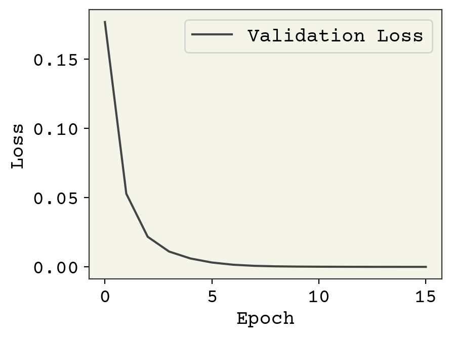
print("final loss value: ", val_loss[-1])
final loss value: tensor(3.6763e-05)
yhat_valuest = [y.detach().numpy() for y in yhat_valuest]
yhat_values = [y.numpy() for y in yhat_values]

yhat_total = np.concatenate([yhat_valuest, yhat_values])
original = feat.numpy()

y_arr = ys.numpy()
yhat_arr = np.stack(yhat_total + original, axis=0)
yhat_vs = np.stack(yhat_values + original[train_split:], axis=0)
y_vs = np.stack(ys[train_split:], axis=0)

yhat_centered = centerofmass(yhat_vs)
y_center = centerofmass(y_vs)
plt.title("centered coordinates")
plt.plot(y_center, y_center, "-")
plt.plot(y_center, yhat_centered, ".")
plt.xlabel("Trajectory")
plt.ylabel("Predicted Trajectory")
plt.annotate(
    "r-squared = {:.3f}".format(r2_score(y_center, yhat_centered)), (11.5, 12.4)
)
plt.show()
Wow! Clearly these parity plots look better than for the baseline model. Let’s again look at the trajectory versus the trajectory predictions, to see visually how they compare. We will look at the training and the validation data together, just note that because the colors represent time, we can look at the purple section to see just the validation data.
fig, axs = plt.subplots(ncols=2, squeeze=True, figsize=(16, 4))

ys_total = np.concatenate([y_st, y_arr])
yhat_st = np.stack(yhatst, axis=0)
yhats_total = np.concatenate([yhat_st, yhat_arr])


axs[0].set_title("Trajectory")
axs[1].set_title("Predicted Trajectory")

cmap = plt.get_cmap("cool")
for i in range(0, 2047, 40):
    axs[0].plot(y_arr[i, :, 0], y_arr[i, :, 1], ".-", alpha=0.2, color=cmap(i / 2047))
    axs[1].plot(
        yhat_arr[i, :, 0], yhat_arr[i, :, 1], ".-", alpha=0.2, color=cmap(i / 2047)
    )
for i in range(2):
    axs[i].set_xticks([])
    axs[i].set_yticks([])
This looks pretty good! Let’s run each model on the last frame to get an extrapolated frame. Remember that for the E3NN model, we predicting displacements, so we’ll just need to add our final displacement back to our final coordinates.
last_frame_bl = y_v
extrp_bl = baseline_model(last_frame_bl, w, b)

last_frame_e3nn = yhat + data.pos
lf_e3nn = []

# format as torch geometric dataset (dummy y values)
lf_e3nn += [
    torch_geometric.data.Data(
        x=None,
        pos=last_frame_e3nn.to(torch.float32),
        y=last_frame_e3nn.to(torch.float32),
    )
]

lf_loader = torch_geometric.loader.DataLoader(lf_e3nn, batch_size=1, shuffle=False)

# run through model
for i in lf_loader:
    extrp_e3nn = model(i)

# add extrapolated displacements back into last frame
extrp_e3nn += last_frame_e3nn
extrp_bl = np.array(extrp_bl)
extrp_e3nn = extrp_e3nn.detach().numpy()

fig, axs = plt.subplots(ncols=2, squeeze=True, figsize=(16, 4))

axs[0].set_title("Baseline Model Extrapolated Frame")
axs[1].set_title("e3nn Model Extrapolated Frame")

cmap = plt.get_cmap("cool")

axs[0].plot(extrp_bl[:, 0], extrp_bl[:, 1], ".-", alpha=0.2)
axs[1].plot(extrp_e3nn[:, 0], extrp_e3nn[:, 1], ".-", alpha=0.2)
for i in range(2):
    axs[i].set_xticks([])
    axs[i].set_yticks([])
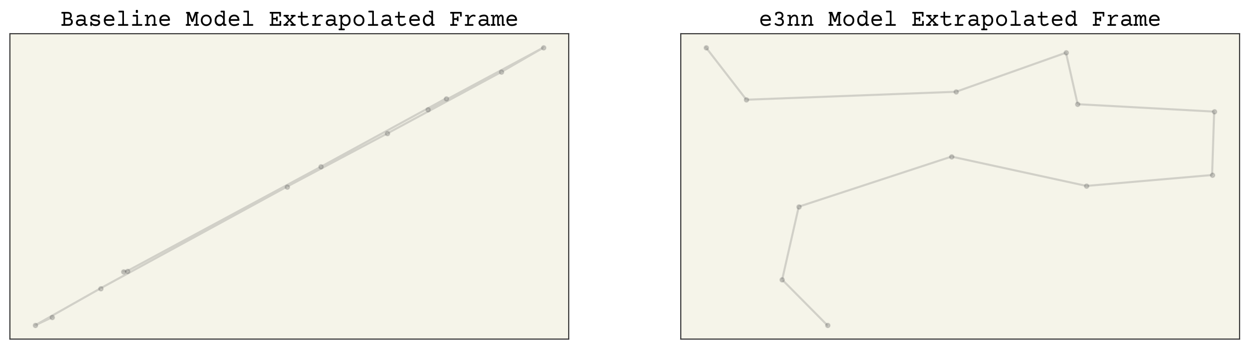
We can clearly see that the e3nn model predicts trajectories much closer to our data. Again, the baseline model has predicted poorly.
Now we can check for equivariance in the same way that we did before with the baseline model. Let’s just take the final frame and rotate, then compare to just the output rotated.
# checking for rotation equivariance
import scipy.spatial.transform as trans

# rotate around x coordinate by 80 degrees
rot = trans.Rotation.from_euler("x", 80, degrees=True)

key3 = jax.random.PRNGKey(58)

input_point = np.asarray(jax.random.normal(key3, (12, 3)))

input_rot = rot.apply(input_point)
input_point = torch.from_numpy(input_point)
input_rot = torch.from_numpy(input_rot)

# format as torch geometric dataset (dummy y values)
rot_first = []
rot_first += [
    torch_geometric.data.Data(
        x=None, pos=input_rot.to(torch.float32), y=input_rot.to(torch.float32)
    )
]
rf_loader = torch_geometric.loader.DataLoader(rot_first, batch_size=1, shuffle=False)
# run through model
for i in rf_loader:
    output_1 = model(i)


# format as torch geometric dataset (dummy y values)
rot_last = []
rot_last += [
    torch_geometric.data.Data(
        x=None, pos=input_point.to(torch.float32), y=input_point.to(torch.float32)
    )
]
rl_loader = torch_geometric.loader.DataLoader(rot_last, batch_size=1, shuffle=False)
# run through model
for i in rl_loader:
    output_2 = model(i)

output_2 = output_2.detach().numpy()
output_1 = output_1.detach().numpy()

output_rot = []
for xyz in output_2:
    coord = rot.apply(xyz)
    output_rot.append(coord)
output_rot = np.array(output_rot)
np.set_printoptions(precision=20, suppress=True)
print("\033[1m" + "difference: " + "\033[0m", np.array([mse(output_1, output_rot)]))

fig, axs = plt.subplots(ncols=2, squeeze=True, figsize=(16, 4))
axs[0].set_title("Translated First")
axs[1].set_title("Translated Last")

for i in range(0, 1, 16):
    axs[0].plot(output_1[:, 0], output_1[:, 1], ".-", alpha=0.2)
    axs[1].plot(output_rot[:, 0], output_rot[:, 1], ".-", alpha=0.2)
for i in range(2):
    axs[i].set_xticks([])
    axs[i].set_yticks([])
difference: [0.00000000000000002197]
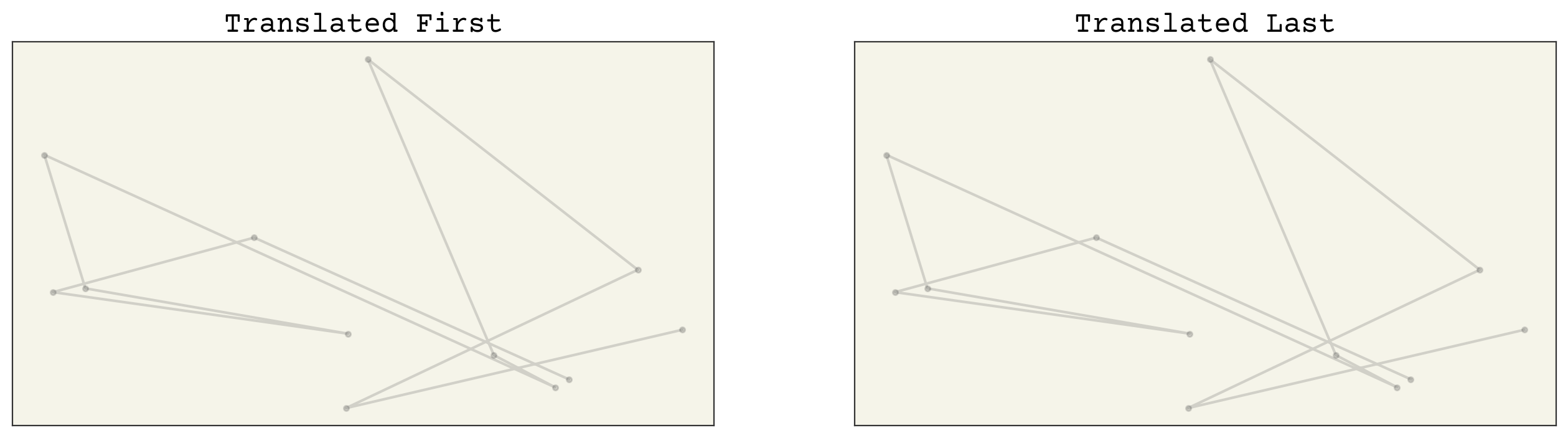
Great! Our random array, when rotated first, gives the same results as when we rotated last! Now we know we have rotational equivariances. I won’t go further to test translational equivariances; I will leave that as an exercise. The E3NN model outperforms the baseline significantly, and it is E(3)-equivariant, unlike our baseline model!
19.6. Cited References#
Mario Geiger and Tess Smidt. E3nn: euclidean neural networks. 2022. URL: https://arxiv.org/abs/2207.09453, doi:10.48550/ARXIV.2207.09453.
Diederik P Kingma and Jimmy Ba. Adam: a method for stochastic optimization. arXiv preprint arXiv:1412.6980, 2014.