23. Modern Molecular NNs

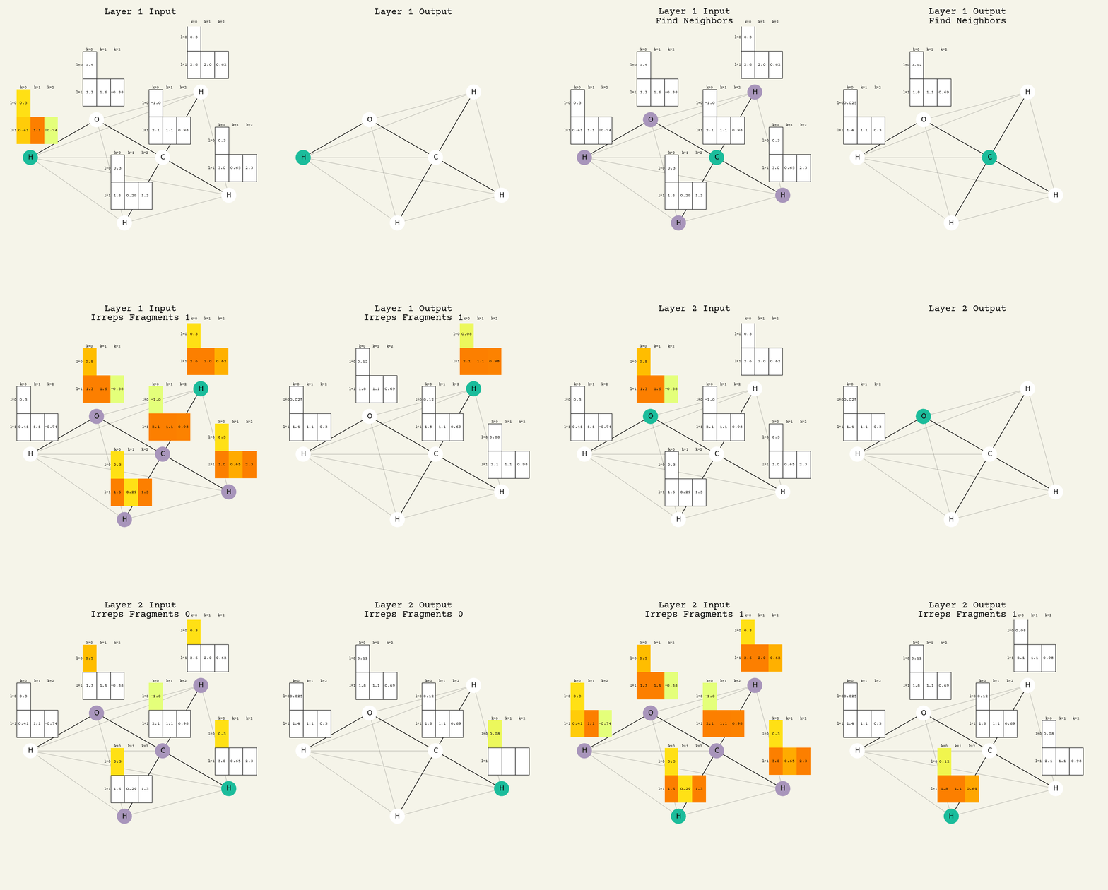
We have seen two chapters about equivariances in Input Data & Equivariances and Equivariant Neural Networks. We have seen one chapter on dealing with molecules as objects with permutation equivariance Graph Neural Networks. We will combine these ideas and create neural networks that can treat arbitrary molecules with point clouds and permutation equivariance. We already saw SchNet is able to do this by working with an invariant point cloud representation (distance to atoms), but modern networks mix in ideas from Equivariant Neural Networks along with graph neural networks (GNN). This is a highly-active research area, especially for predicting energies, forces, and relaxed structures of molecules.

Audience & Objectives

This chapter assumes you have read Input Data & Equivariances, Equivariant Neural Networks, and Graph Neural Networks. You should be able to

• Categorize a task (features/labels) by equivariance

• Understand body-ordered expansions

• Differentiate models based on their message passing, message type, and body-ordering

Warning

This chapter is in progress

24. Expressiveness

The Equivariant SO(3) ideas from Equivariant Neural Networks will not work on variable sized molecules because the layers are not permutation equivariant. We also know that graph neural networks (GNNs) have permutation equivariance and, with the correct choice of edge features, rotation and translation invariance. So why go beyond GNNs?

One reason is that the standard GNNs cannot distinguish certain types of graphs relevant for chemistry is they cannot distinguish molecules like decaline and bicylopentyl, which indeed have different properties. Look at the Fig. 24.1 below and think about the degree and neighbors of the atoms near the mixing of the rings – you’ll see if you try to use message passing the two molecules are identical. This is known as the Wesifeiler-Lehman Test [WL68].

Fig. 24.1 Comparison of decaline and bicylopentyl, which have identical output in most GNNs despite being different molecules.

These can be distinguished if we also have (and use) their Cartesian coordinates. We cannot distinguish enantiomers with GNNs, except maybe with pre-computed node attributes. Even those start to breakdown when we have helical chirality that is not centered at any one molecule.

These are arguments for using Cartesian coordinates in addition to a GNN, but why use equivariant neural networks? Most molnet research is for neural potentials. These are neural networks that predict energy and forces given atom positions and elements. We know that the force on each atom is given by

(24.1)\[\begin{equation} F\left(\vec{r}\right) = -\nabla U\left(\vec{r}\right) \end{equation}\]

where \(U\left(\vec{x}\right)\) is the rotation invariant potential given all atom positions \(\vec{r}\). So if we’re predicting a translation, rotation, and permutation invariant potential, why use equivariance? Part of it is performance. Models like SchNet or ANI are invariant and are not as accurate as models like NequiP or TorchMD-NET that have equivariances in their internal layers. Another reason is that there are indeed specific 3D configurations that should have different energies (according to quantum chemistry calculations), but are invariant if treatd with pairwise distance alone [PC22].

24.1. The Elements of Modern Molecular NNs

There has been a flurry of ideas about molents in the last few years, especially with the advances in equivariant neural network layers. Batatia et al.[BBKovacs+22] have proposed a categorization of the main elements of molnets (which they call E(3)-equivariant NNs) that I will adopt here. They categorize the decisions to be made into three parts of the architecture: the atomic cluster expansions (ACE), the body-order of the messages, and the architecture of the message passing neural network (MPNN). This categorization might also be viewed within the GNN theory as node features (ACE), message creation and aggregation (body-order), and node update (MPNN details). See Graph Neural Networks for more details on MPNNs.

This is a relatively new categorization and certainly is not necessary to use. Most papers do not use this categorization and it takes some effort to put models into it. The benefit of thinking about models with this abstractions is it helps us differentiate between the very large number of models now being pursued in the literature. There is also a bit of chaos in teasing out what differentiates the best models from others. For example, it took a while to discover that the most important features in NequIP were data normalization and how atom embeddings are treated [BBKovacs+22]. This categorization is also improving how these models are designed.

24.1.1. Atom features

Let’s start with the general terminology for an atom. Of course, the input to these networks an atom is just a Cartesian coordinate \(\vec{r}_i\) and the element \(z_i\). As we pass through GNN layers the features will become larger. The atoms are the nodes. The atom features need to be organized a bit differently than previously because some of the features should be invariant with respect to the group — SO(3) — and some need to be equivariant.

24.1.2. Atomic Cluster Expansions

An ACE is a per-atom tensor. The main idea of ACE is to encode the local environment of an atom into a feature tensor that describes its neighborhood of nearby atoms. This is like distinguishing between an oxygen in an alcohol group vs an oxygen in an ether. Both are oxygens, but we expect them to behave differently. ACE is the same idea, but for nearby atoms in space instead of just on the molecular graph.

The general equation for ACE (assuming O(3) equivariance) is [cite]:

(24.2)\[\begin{equation} A^{(t)}_{i, kl_3m_3} = \sum_{l_1m_1,l2_m2}C_{l1m_1,l_2m_2}^{l_3,m_3}\sum_{j \in \mathcal{N}(i)} R^{(t)}_{kl_1l_2l_3}\left(r_{ji}\right)Y_{l1}^{m_1}\left(\hat{\mathbf{r}}_{ji}\right)\mathcal{W}^{(t)}_{kl_2}h_{j,l_2m_2}^{(t)} \end{equation}\]

Wow! What an expression. Let’s go through this carefully, starting with the output. \(A^{(t)}_{i, kl_3m_3}\) are the feature tensor values for atom \(i\) at layer \(t\). There are channels indexed by \(k\) and the spherical harmonic indexes \(l_3m_3\). The right-hand side is nearly identical to the G-equivariant neural network layer equation from Equivariant Neural Networks. We have the input

How is this different than a MPNN

24.2. Normalization

• Physics-based energy/force normalization

• Pooling

• Layers

24.3. Running This Notebook

Click the    above to launch this page as an interactive Google Colab. See details below on installing packages.

Tip

To install packages, execute this code in a new cell.

!pip install dmol-book

If you find install problems, you can get the latest working versions of packages used in this book here

24.4. Cited References

WL68

Boris Weisfeiler and Andrei Leman. The reduction of a graph to canonical form and the algebra which appears therein. NTI, Series, 2(9):12–16, 1968.

PC22

Sergey N Pozdnyakov and Michele Ceriotti. Incompleteness of graph convolutional neural networks for points clouds in three dimensions. arXiv preprint arXiv:2201.07136, 2022.

BBKovacs+22(1,2)

Ilyes Batatia, Simon Batzner, Dávid Péter Kovács, Albert Musaelian, Gregor NC Simm, Ralf Drautz, Christoph Ortner, Boris Kozinsky, and Gábor Csányi. The design space of e (3)-equivariant atom-centered interatomic potentials. arXiv preprint arXiv:2205.06643, 2022.

import matplotlib.pyplot as plt
import matplotlib as mpl
import numpy as np
import tensorflow as tf
import pandas as pd
import rdkit, rdkit.Chem, rdkit.Chem.rdDepictor, rdkit.Chem.Draw
import networkx as nx
import dmol

my_elements = {6: "C", 8: "O", 1: "H"}

def smiles2graph(sml):
    """Argument for the RD2NX function should be a valid SMILES sequence
    returns: the graph
    """
    m = rdkit.Chem.MolFromSmiles(sml)
    m = rdkit.Chem.AddHs(m)
    order_string = {
        rdkit.Chem.rdchem.BondType.SINGLE: 1,
        rdkit.Chem.rdchem.BondType.DOUBLE: 2,
        rdkit.Chem.rdchem.BondType.TRIPLE: 3,
        rdkit.Chem.rdchem.BondType.AROMATIC: 4,
    }
    N = len(list(m.GetAtoms()))
    nodes = np.zeros((N, len(my_elements)))
    lookup = list(my_elements.keys())
    for i in m.GetAtoms():
        nodes[i.GetIdx(), lookup.index(i.GetAtomicNum())] = 1

    adj = np.zeros((N, N, 5))
    for j in m.GetBonds():
        u = min(j.GetBeginAtomIdx(), j.GetEndAtomIdx())
        v = max(j.GetBeginAtomIdx(), j.GetEndAtomIdx())
        order = j.GetBondType()
        if order in order_string:
            order = order_string[order]
        else:
            raise Warning("Ignoring bond order" + order)
        adj[u, v, order] = 1
        adj[v, u, order] = 1
    return nodes, adj

# THIS CELL IS USED TO GENERATE A FIGURE
# AND NOT RELATED TO CHAPTER
# YOU CAN SKIP IT
from myst_nb import glue
from moviepy.editor import VideoClip
from moviepy.video.io.bindings import mplfig_to_npimage


def draw_vector(x, y, s, v, ax, cmap, **kwargs):
    x += s / 2
    y += s / 2
    # iterate vertically
    L = max([len(vi) for vi in v])
    for dy, vi in enumerate(v):
        for dx, vij in enumerate(vi):
            if cmap is not None:
                ax.add_patch(
                    mpl.patches.Rectangle(
                        (x + dx * s * 1.5 / L, y + dy * s),
                        s * 1.5 / L,
                        s,
                        facecolor=cmap(vij),
                        **kwargs,
                    )
                )
            else:
                ax.add_patch(
                    mpl.patches.Rectangle(
                        (x + dx * s * 1.5 / L, y + dy * s),
                        s * 1.5 / L,
                        s,
                        facecolor="#FFF",
                        edgecolor="#333",
                        **kwargs,
                    )
                )
            ax.text(
                x + dx * s * 1.5 / L + s * 1.5 / L / 2,
                y + s / 2 + dy * s,
                "{:.2f}".format(vij),
                verticalalignment="center",
                horizontalalignment="center",
                fontsize=5,
            )


def draw_key(x, y, s, v, ax, cmap, **kwargs):
    x += s / 2
    y += s / 2
    for vi in v:
        ax.add_patch(
            mpl.patches.Rectangle((x, y), s * 1.5, s, facecolor=cmap(1.0), **kwargs)
        )
        ax.text(
            x + s * 1.5 / 2,
            y + s / 2,
            vi,
            verticalalignment="center",
            horizontalalignment="center",
        )
        y += s
    ax.text(
        x, y + s / 2, "Key:", verticalalignment="center", horizontalalignment="left"
    )


def draw(
    nodes,
    node_features,
    adj,
    ax,
    highlight=None,
    key=False,
    labels=None,
    mask=None,
    draw_nodes=None,
):
    G = nx.Graph()
    for i in range(adj.shape[0]):
        for j in range(adj.shape[0]):
            if np.any(adj[i, j]):
                G.add_edge(i, j)
    if mask is None:
        mask = [True] * len(G)
    if draw_nodes is None:
        draw_nodes = nodes
    # go from atomic number to element
    elements = np.argmax(draw_nodes, axis=-1)
    el_labels = {i: list(my_elements.values())[e] for i, e in enumerate(elements)}
    try:
        pos = nx.nx_agraph.graphviz_layout(G, prog="sfdp")
    except ImportError:
        pos = nx.spring_layout(G, iterations=100, seed=4, k=1)
    pos = nx.rescale_layout_dict(pos)
    c = ["white"] * len(G)
    all_h = []
    if highlight is not None:
        for i, h in enumerate(highlight):
            for hj in h:
                c[hj] = "C{}".format(i + 1)
                all_h.append(hj)
    # now we add all edges to close (using pos) atoms to emphasize spatial locality
    for i in range(adj.shape[0]):
        for j in range(adj.shape[0]):
            if (
                i != j
                and not np.any(adj[i, j])
                and np.linalg.norm(np.array(pos[i]) - np.array(pos[j])) < 1
            ):
                G.add_edge(i, j, space=True)
    # set-up edge colors based on if they are space or not
    edge_colors = ["#000"] * len(G.edges)
    for i, (u, v, d) in enumerate(G.edges(data=True)):
        if d.get("space", False):
            edge_colors[i] = "#AAA"
    nx.draw(
        G,
        ax=ax,
        pos=pos,
        labels=el_labels,
        node_size=700,
        node_color=c,
        edge_color=edge_colors,
    )
    cmap = plt.get_cmap("Wistia")
    for i in range(len(G)):
        if not mask[i]:
            continue
        if i in all_h:
            draw_vector(*pos[i], 0.15, node_features[i], ax, cmap)
        else:
            draw_vector(*pos[i], 0.15, node_features[i], ax, None)
    if key:
        draw_key(-1, -1, 0.15, my_elements.values(), ax, cmap)
    if labels is not None:
        legend_elements = []
        for i, l in enumerate(labels):
            p = mpl.lines.Line2D(
                [0], [0], marker="o", color="C{}".format(i + 1), label=l, markersize=15
            )
            legend_elements.append(p)
        ax.legend(handles=legend_elements)
    ax.set_xlim(-1.2, 1.2)
    ax.set_ylim(-1.2, 1.2)
    ax.set_facecolor("#f5f4e9")


nodes, adj = smiles2graph("CO")
print(nodes)
nodes_vectors = [[n, n[:2]] for i, n in enumerate(nodes)]
print(nodes_vectors[1])
fig = plt.figure(figsize=(8, 5))
draw(
    nodes,
    nodes_vectors,
    adj,
    plt.gca(),
    highlight=[[1], [5, 0]],
    labels=["center", "neighbors"],
)
fig.set_facecolor("#f5f4e9")
glue("dframe", plt.gcf(), display=False)

[[1. 0. 0.]
 [0. 1. 0.]
 [0. 0. 1.]
 [0. 0. 1.]
 [0. 0. 1.]
 [0. 0. 1.]]
[array([0., 1., 0.]), array([0., 1.])]

glue("dframe", plt.gcf(), display=False)

# THIS CELL IS USED TO GENERATE A FIGURE
# AND NOT RELATED TO CHAPTER
# YOU CAN SKIP IT
fig, axs = plt.subplots(1, 2, squeeze=True, figsize=(14, 6), dpi=100)
order = [5, 1, 0, 2, 3, 4]
time_per_node = 2
last_layer = [0]
layers = 2
input_nodes = np.copy(nodes)
fig.set_facecolor("#f5f4e9")


def make_frame(t):
    axs[0].clear()
    axs[1].clear()

    layer_i = int(t / (time_per_node * len(order)))
    axs[0].set_title(f"Layer {layer_i + 1} Input")
    axs[1].set_title(f"Layer {layer_i + 1} Output")

    flat_adj = np.sum(adj, axis=-1)
    #     out_nodes = np.einsum(
    #         "i,ij,jk->ik",
    #         1 / (np.sum(flat_adj, axis=1) + 1),
    #         flat_adj + np.eye(*flat_adj.shape),
    #         nodes,
    #     )
    out_nodes = nodes
    node_vectors = [[n, n[:2]] for i, n in enumerate(out_nodes)]
    if last_layer[0] != layer_i:
        print("recomputing")
        nodes[:] = out_nodes
        last_layer[0] = layer_i

    t -= layer_i * time_per_node * len(order)
    i = order[int(t / time_per_node)]
    print(last_layer, layer_i, i, t)
    mask = [False] * nodes.shape[0]
    for j in order[: int(t / time_per_node) + 1]:
        mask[j] = True
    print(mask, i)
    neighs = list(np.where(adj[i])[0])
    if (t - int(t / time_per_node) * time_per_node) >= time_per_node / 4:
        draw(
            nodes,
            node_vectors,
            adj,
            axs[0],
            highlight=[[i], neighs],
            labels=["center", "neighbors"],
            draw_nodes=input_nodes,
        )
    else:
        draw(
            nodes,
            node_vectors,
            adj,
            axs[0],
            highlight=[[i]],
            labels=["center", "neighbors"],
            draw_nodes=input_nodes,
        )
    if (t - int(t / time_per_node) * time_per_node) < time_per_node / 2:
        mask[j] = False
    draw(
        out_nodes,
        node_vectors,
        adj,
        axs[1],
        highlight=[[i]],
        key=True,
        mask=mask,
        draw_nodes=input_nodes,
    )
    fig.set_facecolor("#f5f4e9")
    return mplfig_to_npimage(fig)


animation = VideoClip(make_frame, duration=time_per_node * nodes.shape[0] * layers)
animation.write_gif("../_static/images/molnet.gif", fps=2)

[0] 0 5 0
[False, False, False, False, False, True] 5
MoviePy - Building file ../_static/images/molnet.gif with imageio.

t:   0%|          | 0/48 [00:00<?, ?it/s, now=None]

[0] 0 5 0.0
[False, False, False, False, False, True] 5

t:   4%|▍         | 2/48 [00:00<00:06,  6.62it/s, now=None]

[0] 0 5 0.5
[False, False, False, False, False, True] 5

t:   6%|▋         | 3/48 [00:00<00:09,  4.67it/s, now=None]

[0] 0 5 1.0
[False, False, False, False, False, True] 5

t:   8%|▊         | 4/48 [00:00<00:11,  3.94it/s, now=None]

[0] 0 5 1.5
[False, False, False, False, False, True] 5

t:  10%|█         | 5/48 [00:01<00:11,  3.71it/s, now=None]

[0] 0 1 2.0
[False, True, False, False, False, True] 1

t:  12%|█▎        | 6/48 [00:01<00:11,  3.54it/s, now=None]

[0] 0 1 2.5
[False, True, False, False, False, True] 1

t:  15%|█▍        | 7/48 [00:01<00:11,  3.42it/s, now=None]

[0] 0 1 3.0
[False, True, False, False, False, True] 1

t:  17%|█▋        | 8/48 [00:02<00:11,  3.35it/s, now=None]

[0] 0 1 3.5
[False, True, False, False, False, True] 1

t:  19%|█▉        | 9/48 [00:02<00:11,  3.29it/s, now=None]

[0] 0 0 4.0
[True, True, False, False, False, True] 0

t:  21%|██        | 10/48 [00:02<00:11,  3.19it/s, now=None]

[0] 0 0 4.5
[True, True, False, False, False, True] 0

t:  23%|██▎       | 11/48 [00:03<00:14,  2.60it/s, now=None]

[0] 0 0 5.0
[True, True, False, False, False, True] 0

t:  25%|██▌       | 12/48 [00:03<00:13,  2.73it/s, now=None]

[0] 0 0 5.5
[True, True, False, False, False, True] 0

t:  27%|██▋       | 13/48 [00:03<00:12,  2.84it/s, now=None]

[0] 0 2 6.0
[True, True, True, False, False, True] 2

t:  29%|██▉       | 14/48 [00:04<00:11,  2.93it/s, now=None]

[0] 0 2 6.5
[True, True, True, False, False, True] 2

t:  31%|███▏      | 15/48 [00:04<00:11,  2.93it/s, now=None]

[0] 0 2 7.0
[True, True, True, False, False, True] 2

t:  33%|███▎      | 16/48 [00:04<00:10,  2.96it/s, now=None]

[0] 0 2 7.5
[True, True, True, False, False, True] 2

t:  35%|███▌      | 17/48 [00:05<00:10,  3.01it/s, now=None]

[0] 0 3 8.0
[True, True, True, True, False, True] 3

t:  38%|███▊      | 18/48 [00:05<00:09,  3.00it/s, now=None]

[0] 0 3 8.5
[True, True, True, True, False, True] 3

t:  40%|███▉      | 19/48 [00:05<00:09,  3.00it/s, now=None]

[0] 0 3 9.0
[True, True, True, True, False, True] 3

t:  42%|████▏     | 20/48 [00:06<00:09,  2.98it/s, now=None]

[0] 0 3 9.5
[True, True, True, True, False, True] 3

t:  44%|████▍     | 21/48 [00:06<00:09,  2.96it/s, now=None]

[0] 0 4 10.0
[True, True, True, True, True, True] 4

t:  46%|████▌     | 22/48 [00:07<00:10,  2.44it/s, now=None]

[0] 0 4 10.5
[True, True, True, True, True, True] 4

t:  48%|████▊     | 23/48 [00:07<00:09,  2.60it/s, now=None]

[0] 0 4 11.0
[True, True, True, True, True, True] 4

t:  50%|█████     | 24/48 [00:07<00:08,  2.69it/s, now=None]

[0] 0 4 11.5
[True, True, True, True, True, True] 4

t:  52%|█████▏    | 25/48 [00:08<00:08,  2.75it/s, now=None]

recomputing
[1] 1 5 0.0
[False, False, False, False, False, True] 5

t:  54%|█████▍    | 26/48 [00:08<00:07,  2.89it/s, now=None]

[1] 1 5 0.5
[False, False, False, False, False, True] 5

t:  56%|█████▋    | 27/48 [00:08<00:06,  3.02it/s, now=None]

[1] 1 5 1.0
[False, False, False, False, False, True] 5

t:  58%|█████▊    | 28/48 [00:09<00:06,  3.11it/s, now=None]

[1] 1 5 1.5
[False, False, False, False, False, True] 5

t:  60%|██████    | 29/48 [00:09<00:05,  3.18it/s, now=None]

[1] 1 1 2.0
[False, True, False, False, False, True] 1

t:  62%|██████▎   | 30/48 [00:09<00:05,  3.20it/s, now=None]

[1] 1 1 2.5
[False, True, False, False, False, True] 1

t:  65%|██████▍   | 31/48 [00:10<00:05,  3.23it/s, now=None]

[1] 1 1 3.0
[False, True, False, False, False, True] 1

t:  67%|██████▋   | 32/48 [00:10<00:04,  3.24it/s, now=None]

[1] 1 1 3.5
[False, True, False, False, False, True] 1

t:  69%|██████▉   | 33/48 [00:10<00:04,  3.18it/s, now=None]

[1] 1 0 4.0
[True, True, False, False, False, True] 0

t:  71%|███████   | 34/48 [00:11<00:05,  2.62it/s, now=None]

[1] 1 0 4.5
[True, True, False, False, False, True] 0

t:  73%|███████▎  | 35/48 [00:11<00:04,  2.75it/s, now=None]

[1] 1 0 5.0
[True, True, False, False, False, True] 0

t:  75%|███████▌  | 36/48 [00:11<00:04,  2.85it/s, now=None]

[1] 1 0 5.5
[True, True, False, False, False, True] 0

t:  77%|███████▋  | 37/48 [00:12<00:03,  2.93it/s, now=None]

[1] 1 2 6.0
[True, True, True, False, False, True] 2

t:  79%|███████▉  | 38/48 [00:12<00:03,  3.00it/s, now=None]

[1] 1 2 6.5
[True, True, True, False, False, True] 2

t:  81%|████████▏ | 39/48 [00:12<00:02,  3.02it/s, now=None]

[1] 1 2 7.0
[True, True, True, False, False, True] 2

t:  83%|████████▎ | 40/48 [00:13<00:02,  3.03it/s, now=None]

[1] 1 2 7.5
[True, True, True, False, False, True] 2

t:  85%|████████▌ | 41/48 [00:13<00:02,  3.02it/s, now=None]

[1] 1 3 8.0
[True, True, True, True, False, True] 3

t:  88%|████████▊ | 42/48 [00:13<00:01,  3.00it/s, now=None]

[1] 1 3 8.5
[True, True, True, True, False, True] 3

t:  90%|████████▉ | 43/48 [00:14<00:01,  3.02it/s, now=None]

[1] 1 3 9.0
[True, True, True, True, False, True] 3

t:  92%|█████████▏| 44/48 [00:14<00:01,  3.02it/s, now=None]

[1] 1 3 9.5
[True, True, True, True, False, True] 3

t:  94%|█████████▍| 45/48 [00:15<00:01,  2.47it/s, now=None]

[1] 1 4 10.0
[True, True, True, True, True, True] 4

t:  96%|█████████▌| 46/48 [00:15<00:00,  2.61it/s, now=None]

[1] 1 4 10.5
[True, True, True, True, True, True] 4

t:  98%|█████████▊| 47/48 [00:15<00:00,  2.70it/s, now=None]

[1] 1 4 11.0
[True, True, True, True, True, True] 4

t: 100%|██████████| 48/48 [00:16<00:00,  2.74it/s, now=None]

[1] 1 4 11.5
[True, True, True, True, True, True] 4

<Figure size 900x692.308 with 0 Axes>